
Videos
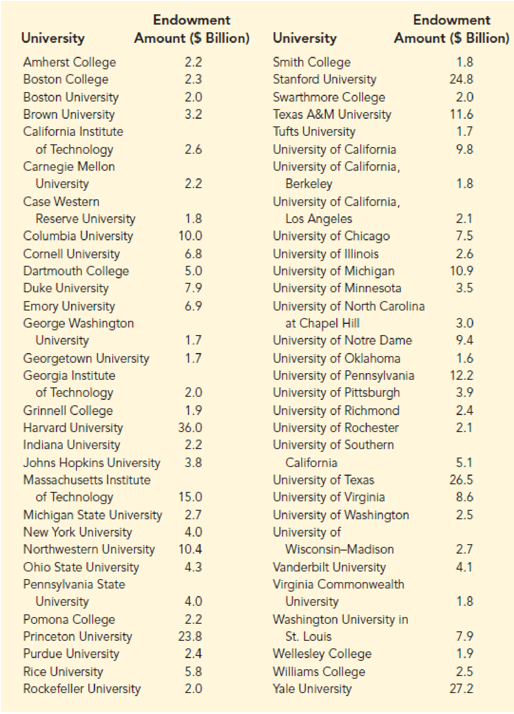
Largest University Endowments. University endowments are financial assets that are donated by supporters to be used to provide income to universities. There is a large discrepancy in the size of university endowments. The following table provides a listing of many of the universities that have the largest endowments as reported by the National Association of College and University Business Officers in 2017.
Summarize the data by constructing the following:
- a. A frequency distribution (classes 0–1.9, 2.0–3.9, 4.0–5.9, 6.0–7.9, and so on).
- b. A relative frequency distribution.
- c. A cumulative frequency distribution.
- d. A cumulative relative frequency distribution.
- e. What do these distributions tell you about the endowments of universities?
- f. Show a histogram. Comment on the shape of the distribution.
- g. What is the largest university endowment and which university holds it?
a.
Construct a frequency distribution for the data.
Answer to Problem 21E
The frequency distribution is as follows:
| Endowment Amount ($ Billion) | Frequency |
| 0-1.9 | 10 |
| 2-3.9 | 24 |
| 4-5.9 | 7 |
| 6-7.9 | 5 |
| 8-9.9 | 3 |
| 10-11.9 | 4 |
| 12-13.9 | 1 |
| 14-15.9 | 1 |
| 16-17.9 | 0 |
| 18-19.9 | 0 |
| 20-21.9 | 0 |
| 22-23.9 | 1 |
| 24-25.9 | 1 |
| 26-27.9 | 2 |
| 28-29.9 | 0 |
| 30-31.9 | 0 |
| 32-33.9 | 0 |
| 34-35.9 | 0 |
| 36-37.9 | 1 |
| Total | 60 |
Explanation of Solution
Calculation:
The data represents the Endowment amount of Universities in billions of dollars and the frequency distribution is constructed using the class 0-1.9, 2-3.9, 4-5.9 and so on.
Frequency:
The frequencies are calculated using the tally mark and the range of the data is from 0 to 37.9.
- Based on the given information, the class intervals are 0-1.9, 2-3.9, 4-5.9, …, 36-37.9.
- Make a tally mark for each value in the corresponding revenue class and continue for all values in the data.
- The number of tally marks in each class represents the frequency, f of that class.
Similarly, the frequency of remaining classes for the Endowment is given below:
| Endowment Amount ($ Billion) | Tally | Frequency |
| 0-1.9 | 10 | |
| 2-3.9 | 24 | |
| 4-5.9 | 7 | |
| 6-7.9 | 5 | |
| 8-9.9 | 3 | |
| 10-11.9 | 4 | |
| 12-13.9 | 1 | |
| 14-15.9 | 1 | |
| 16-17.9 | - | 0 |
| 18-19.9 | - | 0 |
| 20-21.9 | - | 0 |
| 22-23.9 | 1 | |
| 24-25.9 | 1 | |
| 26-27.9 | 2 | |
| 28-29.9 | - | 0 |
| 30-31.9 | - | 0 |
| 32-33.9 | - | 0 |
| 34-35.9 | - | 0 |
| 36-37.9 | 1 | |
| Total | 60 |
b.
Construct a relative frequency distribution for the data.
Answer to Problem 21E
The relative frequency distribution is as follows:
| Endowment Amount ($ Billion) | Frequency | Relative frequency |
| 0-1.9 | 10 | 0.17 |
| 2-3.9 | 24 | 0.40 |
| 4-5.9 | 7 | 0.12 |
| 6-7.9 | 5 | 0.08 |
| 8-9.9 | 3 | 0.05 |
| 10-11.9 | 4 | 0.07 |
| 12-13.9 | 1 | 0.02 |
| 14-15.9 | 1 | 0.02 |
| 16-17.9 | 0 | 0.00 |
| 18-19.9 | 0 | 0.00 |
| 20-21.9 | 0 | 0.00 |
| 22-23.9 | 1 | 0.02 |
| 24-25.9 | 1 | 0.02 |
| 26-27.9 | 2 | 0.03 |
| 28-29.9 | 0 | 0.00 |
| 30-31.9 | 0 | 0.00 |
| 32-33.9 | 0 | 0.00 |
| 34-35.9 | 0 | 0.00 |
| 36-37.9 | 1 | 0.02 |
| Total | 60 | 1 |
Explanation of Solution
Calculation:
Relative frequency:
The general formula for the relative frequency is given below:
For the class (0-1.9), substitute frequency as “10” and total frequency as “60”.
Similarly, the relative frequencies for the remaining Endowment classes are obtained below:
| Endowment Amount ($ Billion) | Frequency | Relative frequency |
| 0-1.9 | 10 | 0.17 |
| 2-3.9 | 24 | 0.40 |
| 4-5.9 | 7 | 0.12 |
| 6-7.9 | 5 | 0.08 |
| 8-9.9 | 3 | 0.05 |
| 10-11.9 | 4 | 0.07 |
| 12-13.9 | 1 | 0.02 |
| 14-15.9 | 1 | 0.02 |
| 16-17.9 | 0 | 0.00 |
| 18-19.9 | 0 | 0.00 |
| 20-21.9 | 0 | 0.00 |
| 22-23.9 | 1 | 0.02 |
| 24-25.9 | 1 | 0.02 |
| 26-27.9 | 2 | 0.03 |
| 28-29.9 | 0 | 0.00 |
| 30-31.9 | 0 | 0.00 |
| 32-33.9 | 0 | 0.00 |
| 34-35.9 | 0 | 0.00 |
| 36-37.9 | 1 | 0.02 |
| Total | 60 | 1 |
c.
Construct a cumulative frequency distribution for the data.
Answer to Problem 21E
The cumulative frequency distribution is as follows:
| Endowment Amount ($ Billion) | Frequency | Cumulative frequency |
| 0-1.9 | 10 | 10 |
| 2-3.9 | 24 | 34 |
| 4-5.9 | 7 | 41 |
| 6-7.9 | 5 | 46 |
| 8-9.9 | 3 | 49 |
| 10-11.9 | 4 | 53 |
| 12-13.9 | 1 | 54 |
| 14-15.9 | 1 | 55 |
| 16-17.9 | 0 | 55 |
| 18-19.9 | 0 | 55 |
| 20-21.9 | 0 | 55 |
| 22-23.9 | 1 | 56 |
| 24-25.9 | 1 | 57 |
| 26-27.9 | 2 | 59 |
| 28-29.9 | 0 | 59 |
| 30-31.9 | 0 | 59 |
| 32-33.9 | 0 | 59 |
| 34-35.9 | 0 | 59 |
| 36-37.9 | 1 | 60 |
Explanation of Solution
Calculation:
Cumulative frequency:
Cumulative frequency of a particular class is the sum of all frequencies up to that class. The last class’s cumulative frequency is equal to the sample size
Thus, the cumulative frequencies for the endowment classes are obtained below:
| Endowment Amount ($ Billion) | Frequency | Cumulative frequency |
| 0-1.9 | 10 | 10 |
| 2-3.9 | 24 | |
| 4-5.9 | 7 | |
| 6-7.9 | 5 | |
| 8-9.9 | 3 | |
| 10-11.9 | 4 | |
| 12-13.9 | 1 | |
| 14-15.9 | 1 | |
| 16-17.9 | 0 | |
| 18-19.9 | 0 | |
| 20-21.9 | 0 | |
| 22-23.9 | 1 | |
| 24-25.9 | 1 | |
| 26-27.9 | 2 | |
| 28-29.9 | 0 | |
| 30-31.9 | 0 | |
| 32-33.9 | 0 | |
| 34-35.9 | 0 | |
| 36-37.9 | 1 |
d.
Construct a cumulative relative frequency distribution for the data.
Answer to Problem 21E
The cumulative relative frequency distribution is given below:
| Endowment Amount ($ Billion) | Frequency | Cumulative Relative Frequency |
| 0-1.9 | 10 | 0.17 |
| 2-3.9 | 24 | 0.57 |
| 4-5.9 | 7 | 0.69 |
| 6-7.9 | 5 | 0.77 |
| 8-9.9 | 3 | 0.82 |
| 10-11.9 | 4 | 0.89 |
| 12-13.9 | 1 | 0.90 |
| 14-15.9 | 1 | 0.92 |
| 16-17.9 | 0 | 0.92 |
| 18-19.9 | 0 | 0.92 |
| 20-21.9 | 0 | 0.92 |
| 22-23.9 | 1 | 0.94 |
| 24-25.9 | 1 | 0.95 |
| 26-27.9 | 2 | 0.99 |
| 28-29.9 | 0 | 0.99 |
| 30-31.9 | 0 | 0.99 |
| 32-33.9 | 0 | 0.99 |
| 34-35.9 | 0 | 0.99 |
| 36-37.9 | 1 | 1.00 |
Explanation of Solution
Calculation:
Cumulative relative frequency of a particular class is the sum of all relative frequencies up to that class. The last class’s cumulative relative frequency is equal to the approximate value 1.00.
The relative frequencies for the endowment classes from part (b) is given below:
| Endowment Amount ($ Billion) | Frequency | Relative frequency |
| 0-1.9 | 10 | 0.17 |
| 2-3.9 | 24 | 0.40 |
| 4-5.9 | 7 | 0.12 |
| 6-7.9 | 5 | 0.08 |
| 8-9.9 | 3 | 0.05 |
| 10-11.9 | 4 | 0.07 |
| 12-13.9 | 1 | 0.02 |
| 14-15.9 | 1 | 0.02 |
| 16-17.9 | 0 | 0.00 |
| 18-19.9 | 0 | 0.00 |
| 20-21.9 | 0 | 0.00 |
| 22-23.9 | 1 | 0.02 |
| 24-25.9 | 1 | 0.02 |
| 26-27.9 | 2 | 0.03 |
| 28-29.9 | 0 | 0.00 |
| 30-31.9 | 0 | 0.00 |
| 32-33.9 | 0 | 0.00 |
| 34-35.9 | 0 | 0.00 |
| 36-37.9 | 1 | 0.02 |
| Total | 60 | 1 |
Thus, the cumulative relative frequencies for the endowment classes are obtained below:
| Endowment Amount ($ Billion) | Relative frequency | Cumulative Relative Frequency |
| 0-1.9 | 0.17 | 0.17 |
| 2-3.9 | 0.40 | |
| 4-5.9 | 0.12 | |
| 6-7.9 | 0.08 | |
| 8-9.9 | 0.05 | |
| 10-11.9 | 0.07 | |
| 12-13.9 | 0.02 | |
| 14-15.9 | 0.02 | |
| 16-17.9 | 0.00 | |
| 18-19.9 | 0.00 | |
| 20-21.9 | 0.00 | |
| 22-23.9 | 0.02 | |
| 24-25.9 | 0.02 | |
| 26-27.9 | 0.03 | |
| 28-29.9 | 0.00 | |
| 30-31.9 | 0.00 | |
| 32-33.9 | 0.00 | |
| 34-35.9 | 0.00 | |
| 36-37.9 | 0.02 | 1.00 |
e.
Explain about the endowment of universities using the distributions.
Explanation of Solution
From the given data set and obtained distributions , it is observed that the frequency for the endowment of universities in the range of 0 billion dollars to less than $16 billion dollars is obtained by majority of 55 Universities over 60 Universities.
Further, the endowment of universities greater $16 billion is obtained by only 5 Universities.
Moreover, 92% of universities have endowment amount under 16 billion dollars. Only 8% of universities have endowment amount over 16 billion dollars.
f.
Construct the histogram and comment on the shape of the distribution.
Answer to Problem 21E
- Output using Excel is given below:
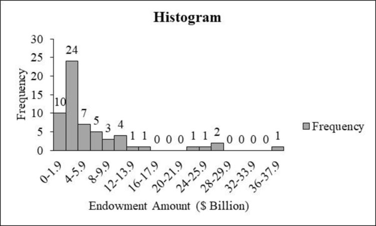
The histogram is skewed to the right.
Explanation of Solution
Calculation:
Step-by-step procedure to draw the frequency histogram chart using Excel is as follows:
- In Excel sheet, enter Endowment Amount ($ Billion) in one column and Frequency in another column.
- Select the data and then choose Insert > Insert Column Bar Charts.
- Select Clustered Column Under More Column Charts.
- Double click the bars
- In Format Data Series, enter 0 in Gap Width under Series Options.
Skewness:
The data is said to be skewed if there is lack of symmetry and values fall on one side that is, either left or right of the distribution.
Right skewed:
If the tail on the distribution is elongated toward the right, more over it attains its peak rapidly than its horizontal axis and then it is a right skewed distribution. It is also called positively skewed.
The distribution of Endowment in the histogram has elongated tail toward right side. There are five universities in the range 20 billion dollars to 37.9 billion dollars.
Therefore, the distribution of the histogram with Endowment is skewed right.
g.
Find the largest university endowment and find the university that holds the largest endowment.
Answer to Problem 21E
The largest university endowment is $36 billion.
The University H holds the largest endowment.
Explanation of Solution
From the data set of 60 universities, it is observed that the largest university endowment is $36 billion and the university is University H.
Moreover, the endowment of remaining universities has less than 28 billion dollars and most of the universities have less than 16 billion dollars and is approximately 92 percent.
Want to see more full solutions like this?
Chapter 2 Solutions
Essentials of Statistics for Business and Economics


- Exercise 6-6 (Algo) (LO6-3) The director of admissions at Kinzua University in Nova Scotia estimated the distribution of student admissions for the fall semester on the basis of past experience. Admissions Probability 1,100 0.5 1,400 0.4 1,300 0.1 Click here for the Excel Data File Required: What is the expected number of admissions for the fall semester? Compute the variance and the standard deviation of the number of admissions. Note: Round your standard deviation to 2 decimal places.arrow_forward1. Find the mean of the x-values (x-bar) and the mean of the y-values (y-bar) and write/label each here: 2. Label the second row in the table using proper notation; then, complete the table. In the fifth and sixth columns, show the 'products' of what you're multiplying, as well as the answers. X y x minus x-bar y minus y-bar (x minus x-bar)(y minus y-bar) (x minus x-bar)^2 xy 16 20 34 4-2 5 2 3. Write the sums that represents Sxx and Sxy in the table, at the bottom of their respective columns. 4. Find the slope of the Regression line: bi = (simplify your answer) 5. Find the y-intercept of the Regression line, and then write the equation of the Regression line. Show your work. Then, BOX your final answer. Express your line as "y-hat equals...arrow_forwardApply STATA commands & submit the output for each question only when indicated below i. Generate the log of birthweight and family income of children. Name these new variables Ibwght & Ifaminc. Include the output of this code. ii. Apply the command sum with the detail option to the variable faminc. Note: you should find the 25th percentile value, the 50th percentile and the 75th percentile value of faminc from the output - you will need it to answer the next question Include the output of this code. iii. iv. Use the output from part ii of this question to Generate a variable called "high_faminc" that takes a value 1 if faminc is less than or equal to the 25th percentile, it takes the value 2 if faminc is greater than 25th percentile but less than or equal to the 50th percentile, it takes the value 3 if faminc is greater than 50th percentile but less than or equal to the 75th percentile, it takes the value 4 if faminc is greater than the 75th percentile. Include the outcome of this code…arrow_forward
- solve this on paperarrow_forwardApply STATA commands & submit the output for each question only when indicated below i. Apply the command egen to create a variable called "wyd" which is the rowtotal function on variables bwght & faminc. ii. Apply the list command for the first 10 observations to show that the code in part i worked. Include the outcome of this code iii. Apply the egen command to create a new variable called "bwghtsum" using the sum function on variable bwght by the variable high_faminc (Note: need to apply the bysort' statement) iv. Apply the "by high_faminc" statement to find the V. descriptive statistics of bwght and bwghtsum Include the output of this code. Why is there a difference between the standard deviations of bwght and bwghtsum from part iv of this question?arrow_forwardAccording to a health information website, the distribution of adults’ diastolic blood pressure (in millimeters of mercury, mmHg) can be modeled by a normal distribution with mean 70 mmHg and standard deviation 20 mmHg. b. Above what diastolic pressure would classify someone in the highest 1% of blood pressures? Show all calculations used.arrow_forward
- Write STATA codes which will generate the outcomes in the questions & submit the output for each question only when indicated below i. ii. iii. iv. V. Write a code which will allow STATA to go to your favorite folder to access your files. Load the birthweight1.dta dataset from your favorite folder and save it under a different filename to protect data integrity. Call the new dataset babywt.dta (make sure to use the replace option). Verify that it contains 2,998 observations and 8 variables. Include the output of this code. Are there missing observations for variable(s) for the variables called bwght, faminc, cigs? How would you know? (You may use more than one code to show your answer(s)) Include the output of your code (s). Write the definitions of these variables: bwght, faminc, male, white, motheduc,cigs; which of these variables are categorical? [Hint: use the labels of the variables & the browse command] Who is this dataset about? Who can use this dataset to answer what kind of…arrow_forwardApply STATA commands & submit the output for each question only when indicated below İ. ii. iii. iv. V. Apply the command summarize on variables bwght and faminc. What is the average birthweight of babies and family income of the respondents? Include the output of this code. Apply the tab command on the variable called male. How many of the babies and what share of babies are male? Include the output of this code. Find the summary statistics (i.e. use the sum command) of the variables bwght and faminc if the babies are white. Include the output of this code. Find the summary statistics (i.e. use the sum command) of the variables bwght and faminc if the babies are male but not white. Include the output of this code. Using your answers to previous subparts of this question: What is the difference between the average birthweight of a baby who is male and a baby who is male but not white? What can you say anything about the difference in family income of the babies that are male and male…arrow_forwardA public health researcher is studying the impacts of nudge marketing techniques on shoppers vegetablesarrow_forward
- The director of admissions at Kinzua University in Nova Scotia estimated the distribution of student admissions for the fall semester on the basis of past experience. Admissions Probability 1,100 0.5 1,400 0.4 1,300 0.1 Click here for the Excel Data File Required: What is the expected number of admissions for the fall semester? Compute the variance and the standard deviation of the number of admissions. Note: Round your standard deviation to 2 decimal places.arrow_forwardA pollster randomly selected four of 10 available people. Required: How many different groups of 4 are possible? What is the probability that a person is a member of a group? Note: Round your answer to 3 decimal places.arrow_forwardWind Mountain is an archaeological study area located in southwestern New Mexico. Potsherds are broken pieces of prehistoric Native American clay vessels. One type of painted ceramic vessel is called Mimbres classic black-on-white. At three different sites the number of such sherds was counted in local dwelling excavations. Test given. Site I Site II Site III 63 19 60 43 34 21 23 49 51 48 11 15 16 46 26 20 31 Find .arrow_forward
 Glencoe Algebra 1, Student Edition, 9780079039897...AlgebraISBN:9780079039897Author:CarterPublisher:McGraw Hill
 Big Ideas Math A Bridge To Success Algebra 1: Stu...AlgebraISBN:9781680331141Author:HOUGHTON MIFFLIN HARCOURTPublisher:Houghton Mifflin Harcourt
 Holt Mcdougal Larson Pre-algebra: Student Edition...AlgebraISBN:9780547587776Author:HOLT MCDOUGALPublisher:HOLT MCDOUGAL