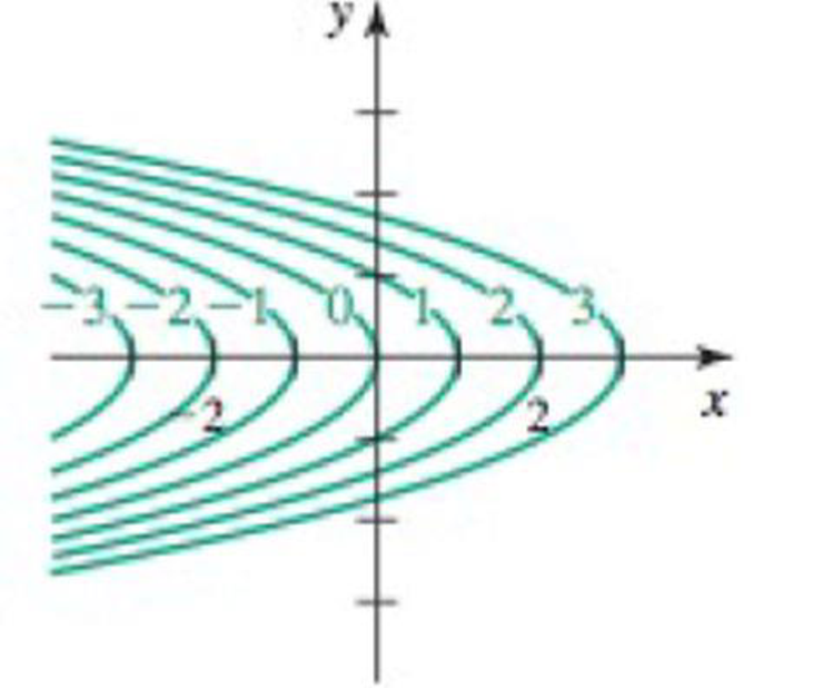
Equipotential curves Consider the following potential functions and graphs of their equipotential curves. a. Find the associated gradient field F = ▿ ϕ. b. Show that the vector field is orthogonal to the equipotential curve at the point (1, 1) . Illustrate this result on the figure. c. Show that the vector field is orthogonal to the equipotential curve at all points ( x, y ). d. Sketch two flow curves representing F that are everywhere orthogonal to the equipotential curves. 38. ϕ ( x, y ) = x + y 2
Equipotential curves Consider the following potential functions and graphs of their equipotential curves. a. Find the associated gradient field F = ▿ ϕ. b. Show that the vector field is orthogonal to the equipotential curve at the point (1, 1) . Illustrate this result on the figure. c. Show that the vector field is orthogonal to the equipotential curve at all points ( x, y ). d. Sketch two flow curves representing F that are everywhere orthogonal to the equipotential curves. 38. ϕ ( x, y ) = x + y 2
Solution Summary: The author explains the gradient field for the potential function phi (x,y)=x+y2. The vector field is orthogonal to the equipotential curve.
Equipotential curves Consider the following potential functions and graphs of their equipotential curves.
a. Find the associated gradient fieldF= ▿ϕ.
b. Show that the vector field is orthogonal to the equipotential curve at the point (1, 1). Illustrate this result on the figure.
c. Show that the vector field is orthogonal to the equipotential curve at all points (x, y).
d. Sketch two flow curves representingF that are everywhere orthogonal to the equipotential curves.
38.ϕ (x, y) = x + y2
Quantities that have magnitude and direction but not position. Some examples of vectors are velocity, displacement, acceleration, and force. They are sometimes called Euclidean or spatial vectors.
Good Day,
Kindly assist with the following query.
Regards,
Example 1
Solve the following differential equations:
dy
dx
ex
= 3x²-6x+5
dy
dx
= 4,
y(0) = 3
x
dy
dx
33
= 5x3 +4
Prof. Robdera
5
-10:54 1x ㅁ +
21. First-Order Constant-Coefficient Equations.
a. Substituting y = ert, find the auxiliary equation for the first-order linear
equation
ay+by = 0,
where a and b are constants with a 0.
b. Use the result of part (a) to find the general solution.
University Calculus: Early Transcendentals (4th Edition)
Knowledge Booster
Learn more about
Need a deep-dive on the concept behind this application? Look no further. Learn more about this topic, calculus and related others by exploring similar questions and additional content below.
01 - What Is an Integral in Calculus? Learn Calculus Integration and how to Solve Integrals.; Author: Math and Science;https://www.youtube.com/watch?v=BHRWArTFgTs;License: Standard YouTube License, CC-BY


 Algebra & Trigonometry with Analytic GeometryAlgebraISBN:9781133382119Author:SwokowskiPublisher:Cengage
 Algebra and Trigonometry (MindTap Course List)AlgebraISBN:9781305071742Author:James Stewart, Lothar Redlin, Saleem WatsonPublisher:Cengage Learning