
Videos
The article first introduced in Exercise 13.34 of Section 13.3 gave data on the dimensions of 27 representative food products.
- a. Use the data set given there to test the hypothesis that there is a positive linear relationship between x = minimum width and y = maximum width of an object.
- b. Calculate and interpret se.
- c. Calculate a 95% confidence interval for the mean maximum width of products with a minimum width of 6 cm.
- d. Calculate a 95% prediction interval for the maximum width of a food package with a minimum width of 6 cm.
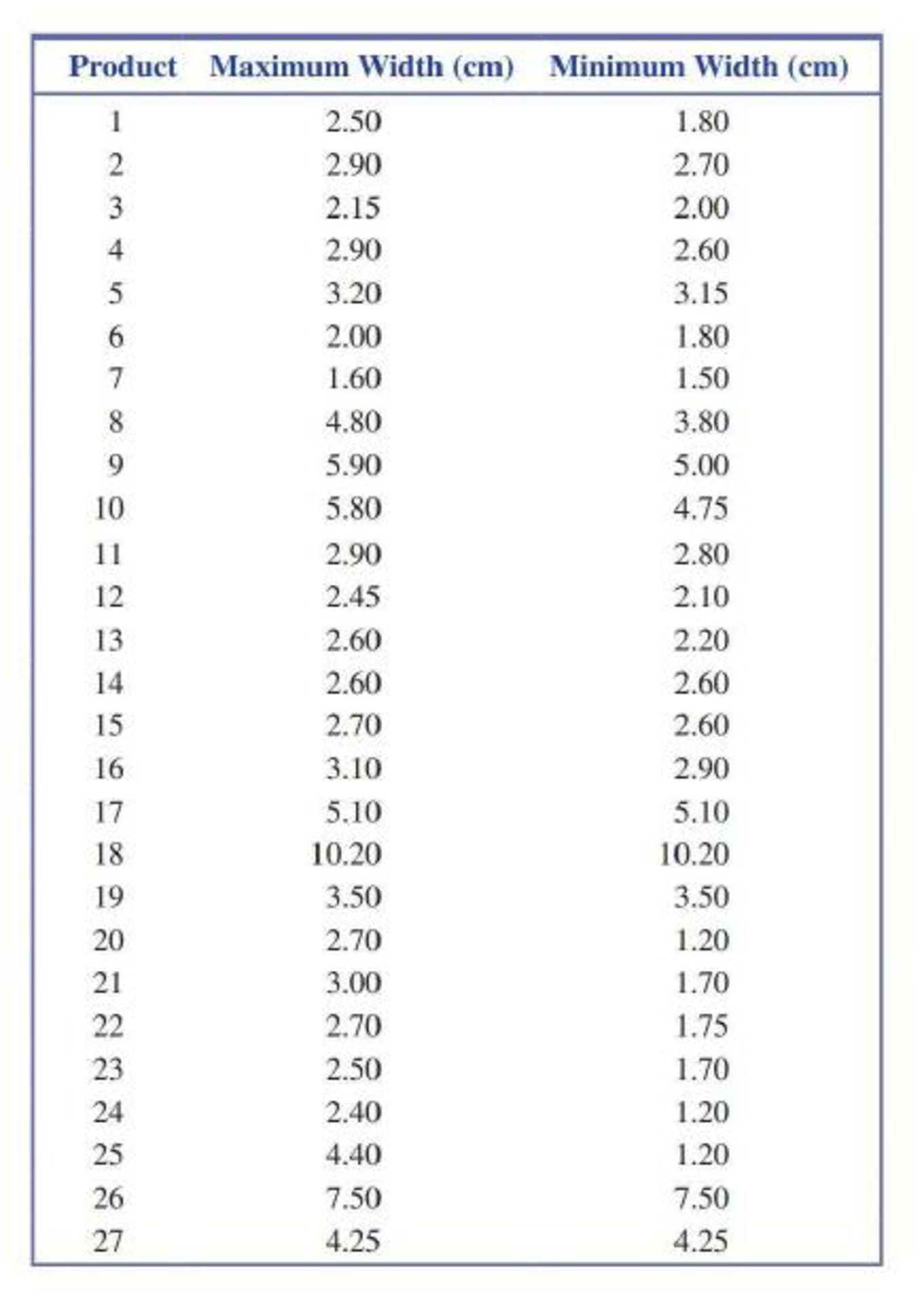
13.34 The article “Vital Dimensions in Volume Perception: Can the Eye Fool the Stomach?” (Journal of Marketing Research [1999]: 313–326) gave the accompanying data on the dimensions of 27 representative food products (Gerber baby food, Cheez Whiz, Skippy Peanut Butter, and Ahmed’s tandoori paste, to name a few).
- a. Fit the simple linear regression model that would allow prediction of the maximum width of a food container based on its minimum width.
- b. Calculate the standardized residuals (or just the residuals if a computer program that doesn’t give standardized residuals is used) and make a residual plot to determine whether there are any outliers.
- c. The data point with the largest residual is for a 1-liter Coke bottle. Delete this data point and determine the equation of the regression line. Did deletion of this point result in a large change in the equation of the estimated regression line?
- d. For the regression line of Part (c), interpret the estimated slope and, if appropriate, the intercept.
- e. For the data set with the Coke bottle deleted, are the assumptions of the simple linear regression model reasonable? Give statistical evidence.
a.
Check whether there is a positive linear relationship between minimum and maximum width of an object.
Answer to Problem 44E
There is convincing evidence that there is a positive linear relationship between minimum and maximum width of an object.
Explanation of Solution
Calculation:
The given data provide the dimensions of 27 representative food products.
1.
Here,
2.
Null hypothesis:
That is, there is no linear relationship between minimum and maximum width of an object.
3.
Alternative hypothesis:
That is, there is a positive linear relationship between minimum and maximum width of an object.
4.
Here, the significance level is
5.
Test Statistic:
The formula for test statistic is,
In the formula, b denotes the estimated slope,
6.
A standardized residual plot is shown below.
Standardized residual values and standardized residual plot:
Software procedure:
Step-by-step procedure to compute standardized residuals and its plot using MINITAB software:
- Select Stat > Regression > Regression > Fit Regression Model
- In Response, enter the column of Maximum width.
- In Continuous Predictors, enter the columns of Minimum width.
- In Graphs, select Standardized under Residuals for Plots.
- In Results, select for all observations under Fits and diagnostics.
- In Residuals versus the variables, select Minimum width.
- Click OK.
Output obtained the MINTAB software is given below:
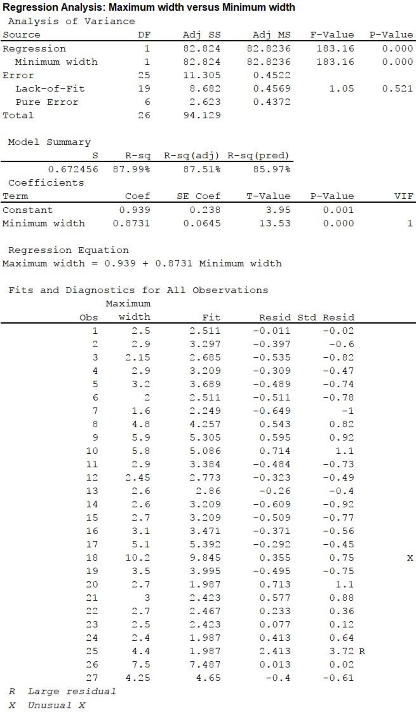
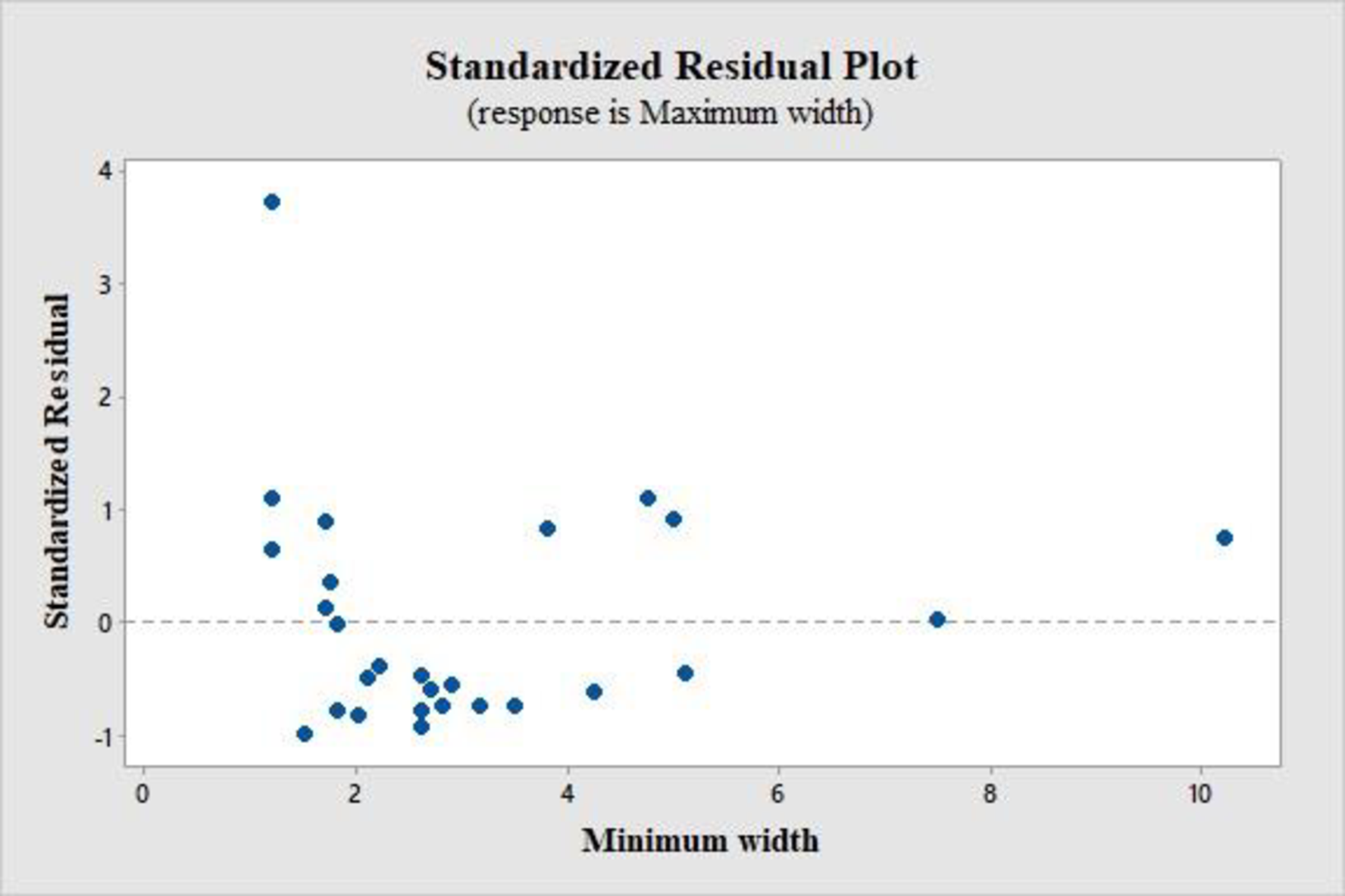
From the standardized residual plot, it is observed that one point lies outside the horizontal band of 3 units from the central line of 0. The standardized residual for this outlier is 3.72, which is for the product 25.
Assumption:
Here, the assumption made is that, the simple linear regression model is appropriate for the data, even though there is one extreme standardized residual.
7.
Calculation:
Test Statistic:
In the MINITAB output, the test statistic value is displayed in the column “T-value” corresponding to “Minimum width”, in the section “Coefficients”. The value is 13.53.
8.
P-value:
From the above output, the correponding P-value is 0.
9.
Rejection rule:
If
Conclusion:
The P-value is 0.
The level of significance is 0.05.
The P-value is less than the level of significance.
That is,
Based on the rejection rule, reject the null hypothesis.
Thus, there is convincing evidence that there is a positive linear relationship between minimum and maximum width of an object.
b.
Compute and interpret
Answer to Problem 44E
Explanation of Solution
Calculation:
From the MINITAB output in Part (a), it is clear that
On an average, there is a 67.246% deviation of the maximum width in the sample from the value predicted by least-squares regression.
c.
Find the 95% confidence interval for the mean maximum width of products, for a minimum width of 6 cm.
Answer to Problem 44E
The 95% interval for the mean maximum width of products, for a minimum width of 6 cm is (5.708, 6.647).
Explanation of Solution
Calculation:
The confidence interval for
From the MINITAB output in Part (a), the estimated linear regression line is
Point estimate:
The point estimate is calculated as follows.
Estimated standard deviation:
For the given x values, the summation values are given in the following table.
| Minimum width (X) | |
| 1.8 | 3.24 |
| 2.7 | 7.29 |
| 2 | 4 |
| 2.6 | 6.76 |
| 3.15 | 9.9225 |
| 1.8 | 3.24 |
| 1.5 | 2.25 |
| 3.8 | 14.44 |
| 5 | 25 |
| 4.75 | 22.5625 |
| 2.8 | 7.84 |
| 2.1 | 4.41 |
| 2.2 | 4.84 |
| 2.6 | 6.76 |
| 2.6 | 6.76 |
| 2.9 | 8.41 |
| 5.1 | 26.01 |
| 10.2 | 104.04 |
| 3.5 | 12.25 |
| 1.2 | 1.44 |
| 1.7 | 2.89 |
| 1.75 | 3.0625 |
| 1.7 | 2.89 |
| 1.2 | 1.44 |
| 1.2 | 1.44 |
| 7.5 | 56.25 |
| 4.25 | 18.0625 |
The value of
Substitute,
Formula for Degrees of freedom:
The formula for degrees of freedom is,
The number of data values given is 27, that is
Critical value:
From the Appendix: Table of t Critical Values:
- Locate the value 25 in the degrees of freedom (df) column.
- Locate the 0.95 in the row of central area captured.
- The intersecting value that corresponds to the df 25 with confidence level 0.95 is 2.060.
Thus, the critical value for
Substitute,
Therefore, one can be 95% confident that the mean maximum width of products with a minimum width of 6 cm will be between 5.708 cm and 6.647 cm.
d.
Find a 95% prediction interval for the mean maximum width of products with a minimum width of 6 cm.
Answer to Problem 44E
The 95% prediction interval for the mean maximum width of products with a minimum width of 6 cm is (4.716, 7.640).
Explanation of Solution
Calculation:
The confidence interval for
The estimated standard deviation of the amount by which a single y observation deviates from the value predicted by an estimated regression line is,
Substitute
From Part (c), the critical value for
Substitute,
Therefore, the 95% prediction interval for the mean maximum width of products with a minimum width of 6 cm is (4.716, 7.640).
Want to see more full solutions like this?
Chapter 13 Solutions
Introduction To Statistics And Data Analysis


- Question 1 The data shown in Table 1 are and R values for 24 samples of size n = 5 taken from a process producing bearings. The measurements are made on the inside diameter of the bearing, with only the last three decimals recorded (i.e., 34.5 should be 0.50345). Table 1: Bearing Diameter Data Sample Number I R Sample Number I R 1 34.5 3 13 35.4 8 2 34.2 4 14 34.0 6 3 31.6 4 15 37.1 5 4 31.5 4 16 34.9 7 5 35.0 5 17 33.5 4 6 34.1 6 18 31.7 3 7 32.6 4 19 34.0 8 8 33.8 3 20 35.1 9 34.8 7 21 33.7 2 10 33.6 8 22 32.8 1 11 31.9 3 23 33.5 3 12 38.6 9 24 34.2 2 (a) Set up and R charts on this process. Does the process seem to be in statistical control? If necessary, revise the trial control limits. [15 pts] (b) If specifications on this diameter are 0.5030±0.0010, find the percentage of nonconforming bearings pro- duced by this process. Assume that diameter is normally distributed. [10 pts] 1arrow_forward4. (5 pts) Conduct a chi-square contingency test (test of independence) to assess whether there is an association between the behavior of the elderly person (did not stop to talk, did stop to talk) and their likelihood of falling. Below, please state your null and alternative hypotheses, calculate your expected values and write them in the table, compute the test statistic, test the null by comparing your test statistic to the critical value in Table A (p. 713-714) of your textbook and/or estimating the P-value, and provide your conclusions in written form. Make sure to show your work. Did not stop walking to talk Stopped walking to talk Suffered a fall 12 11 Totals 23 Did not suffer a fall | 2 Totals 35 37 14 46 60 Tarrow_forwardQuestion 2 Parts manufactured by an injection molding process are subjected to a compressive strength test. Twenty samples of five parts each are collected, and the compressive strengths (in psi) are shown in Table 2. Table 2: Strength Data for Question 2 Sample Number x1 x2 23 x4 x5 R 1 83.0 2 88.6 78.3 78.8 3 85.7 75.8 84.3 81.2 78.7 75.7 77.0 71.0 84.2 81.0 79.1 7.3 80.2 17.6 75.2 80.4 10.4 4 80.8 74.4 82.5 74.1 75.7 77.5 8.4 5 83.4 78.4 82.6 78.2 78.9 80.3 5.2 File Preview 6 75.3 79.9 87.3 89.7 81.8 82.8 14.5 7 74.5 78.0 80.8 73.4 79.7 77.3 7.4 8 79.2 84.4 81.5 86.0 74.5 81.1 11.4 9 80.5 86.2 76.2 64.1 80.2 81.4 9.9 10 75.7 75.2 71.1 82.1 74.3 75.7 10.9 11 80.0 81.5 78.4 73.8 78.1 78.4 7.7 12 80.6 81.8 79.3 73.8 81.7 79.4 8.0 13 82.7 81.3 79.1 82.0 79.5 80.9 3.6 14 79.2 74.9 78.6 77.7 75.3 77.1 4.3 15 85.5 82.1 82.8 73.4 71.7 79.1 13.8 16 78.8 79.6 80.2 79.1 80.8 79.7 2.0 17 82.1 78.2 18 84.5 76.9 75.5 83.5 81.2 19 79.0 77.8 20 84.5 73.1 78.2 82.1 79.2 81.1 7.6 81.2 84.4 81.6 80.8…arrow_forward
- Name: Lab Time: Quiz 7 & 8 (Take Home) - due Wednesday, Feb. 26 Contingency Analysis (Ch. 9) In lab 5, part 3, you will create a mosaic plot and conducted a chi-square contingency test to evaluate whether elderly patients who did not stop walking to talk (vs. those who did stop) were more likely to suffer a fall in the next six months. I have tabulated the data below. Answer the questions below. Please show your calculations on this or a separate sheet. Did not stop walking to talk Stopped walking to talk Totals Suffered a fall Did not suffer a fall Totals 12 11 23 2 35 37 14 14 46 60 Quiz 7: 1. (2 pts) Compute the odds of falling for each group. Compute the odds ratio for those who did not stop walking vs. those who did stop walking. Interpret your result verbally.arrow_forwardSolve please and thank you!arrow_forward7. In a 2011 article, M. Radelet and G. Pierce reported a logistic prediction equation for the death penalty verdicts in North Carolina. Let Y denote whether a subject convicted of murder received the death penalty (1=yes), for the defendant's race h (h1, black; h = 2, white), victim's race i (i = 1, black; i = 2, white), and number of additional factors j (j = 0, 1, 2). For the model logit[P(Y = 1)] = a + ß₁₂ + By + B²², they reported = -5.26, D â BD = 0, BD = 0.17, BY = 0, BY = 0.91, B = 0, B = 2.02, B = 3.98. (a) Estimate the probability of receiving the death penalty for the group most likely to receive it. [4 pts] (b) If, instead, parameters used constraints 3D = BY = 35 = 0, report the esti- mates. [3 pts] h (c) If, instead, parameters used constraints Σ₁ = Σ₁ BY = Σ; B = 0, report the estimates. [3 pts] Hint the probabilities, odds and odds ratios do not change with constraints.arrow_forward
- Solve please and thank you!arrow_forwardSolve please and thank you!arrow_forwardQuestion 1:We want to evaluate the impact on the monetary economy for a company of two types of strategy (competitive strategy, cooperative strategy) adopted by buyers.Competitive strategy: strategy characterized by firm behavior aimed at obtaining concessions from the buyer.Cooperative strategy: a strategy based on a problem-solving negotiating attitude, with a high level of trust and cooperation.A random sample of 17 buyers took part in a negotiation experiment in which 9 buyers adopted the competitive strategy, and the other 8 the cooperative strategy. The savings obtained for each group of buyers are presented in the pdf that i sent: For this problem, we assume that the samples are random and come from two normal populations of unknown but equal variances.According to the theory, the average saving of buyers adopting a competitive strategy will be lower than that of buyers adopting a cooperative strategy.a) Specify the population identifications and the hypotheses H0 and H1…arrow_forward
- You assume that the annual incomes for certain workers are normal with a mean of $28,500 and a standard deviation of $2,400. What’s the chance that a randomly selected employee makes more than $30,000?What’s the chance that 36 randomly selected employees make more than $30,000, on average?arrow_forwardWhat’s the chance that a fair coin comes up heads more than 60 times when you toss it 100 times?arrow_forwardSuppose that you have a normal population of quiz scores with mean 40 and standard deviation 10. Select a random sample of 40. What’s the chance that the mean of the quiz scores won’t exceed 45?Select one individual from the population. What’s the chance that his/her quiz score won’t exceed 45?arrow_forward
 Linear Algebra: A Modern IntroductionAlgebraISBN:9781285463247Author:David PoolePublisher:Cengage Learning
 Glencoe Algebra 1, Student Edition, 9780079039897...AlgebraISBN:9780079039897Author:CarterPublisher:McGraw Hill
 Big Ideas Math A Bridge To Success Algebra 1: Stu...AlgebraISBN:9781680331141Author:HOUGHTON MIFFLIN HARCOURTPublisher:Houghton Mifflin Harcourt