Chapter 13, Problem 60CR

The article “Photocharge Effects in Dye Sensitized Ag[Br, I] Emulsions at Millisecond Range Exposures” (Photographic Science and Engineering [1981]: 138–144) gave the accompanying data on x = Percentage of light absorption and y = Peak photovoltage.

1. a. Construct a scatterplot of the data. What does it suggest?
2. b. Assuming that the simple linear regression model is appropriate, obtain the equation of the estimated regression line.
3. c. How much of the observed variation in peak photovoltage can be explained by the model relationship?
4. d. Predict peak photovoltage when percent absorption is 19.1, and compute the value of the corresponding residual.
5. e. The authors claimed that there is a useful linear relationship between the two variables. Do you agree? Carry out a formal test.
6. f. Give an estimate of the average change in peak photovoltage associated with a 1 percentage point increase in light absorption. Your estimate should convey information about the precision of estimation.
7. g. Give an estimate of mean peak photovoltage when percentage of light absorption is 20, and do so in a way that conveys information about precision.

To determine

Construct a scatterplot for the data and explain what it suggests.

Explanation of Solution

Calculation:

The given data are on percentage of light absorption (x) and peak photo voltage (y).

If the scatterplot of the data shows a linear pattern, and the vertical variability of points does not appear to be changing over the range of x values in the sample, then it can be said that the data is consistent with the use of the simple linear regression model.

Software procedure:

Step-by-step procedure to obtain the scatterplot using MINITAB software:

• Choose Graph > Scatter plot.
• Select Simple.
• Click OK.
• Under Y variables, enter the column of y.
• Under X variables, enter the column of x.
• Click OK.

The output using MINITAB software is given below:

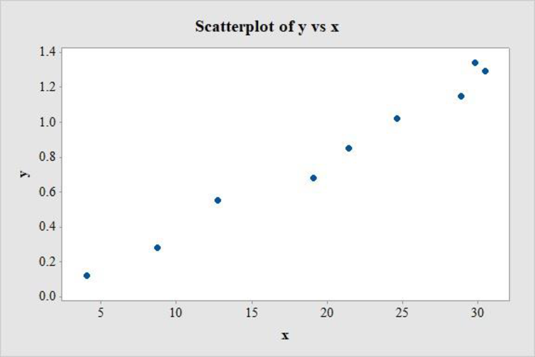
The scatter plot shows no apparent curve and there are no extreme observations. There is no change in the y values as the values of x change and there are no influential points. Therefore, the simple linear regression model seems appropriate for the data set.

To determine

Find the equation of the estimated regression line by assuming that the simple linear regression model is appropriate.

Answer to Problem 60CR

The equation of the estimated regression line is, $\widehat{y}=-0.0826+0.0446x$.

Explanation of Solution

Calculation:

Regression Analysis:

Software procedure:

Step-by-step procedure to obtain the regression line using MINITAB software:

• Choose Stat > Regression > Regression > Fit Regression Model.
• Under Responses, enter the column of values y.
• Under Continuous predictors, enter the column of values x.
• Click OK.

Output using MINITAB software is given below:

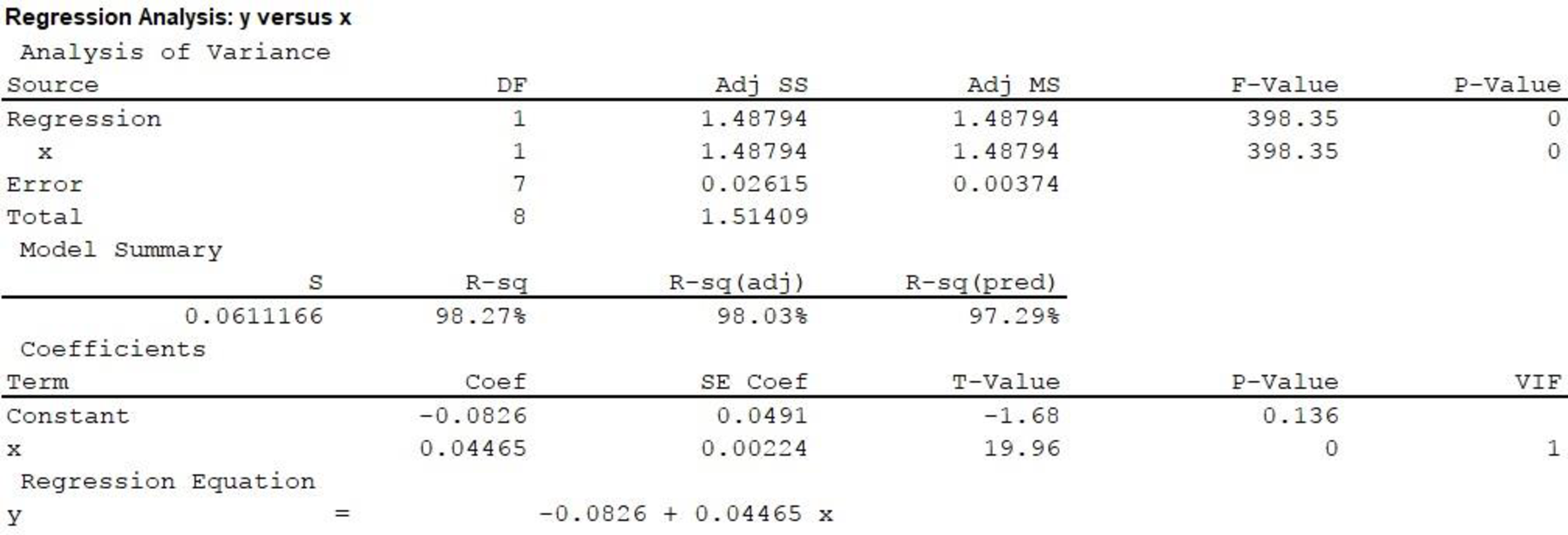
Hence, the equation of the estimated regression line by assuming that the simple linear regression model is appropriate is, $\widehat{y}=-0.0826+0.0446x$.

To determine

Find how much of the observed variation in peak photo voltage can be explained by the model relationship.

Answer to Problem 60CR

The percentage of observed variation in peak photo voltage that can be explained by the model relationship is 98.3%.

Explanation of Solution

From the Minitab output in Part (b), the value of $r^2$ is 98.27%.

This implies that 98.27%, or approximately 98.3% of the observed variation in the dependent variable ‘peak photo voltage’ is being explained by the independent variable ‘percentage of light absorption’ using the simple linear regression model. The change is attributable to the linear relationship between the variables ‘peak photo voltage’ and ‘percentage of light absorption’ and is being explained by the model.

Thus, the percentage of observed variation in peak photo voltage that can be explained by the model relationship is 98.3%.

To determine

Predict peak photo voltage when percent absorption is 19.1.

Find the value of the corresponding residual.

Answer to Problem 60CR

The peak voltage when percent absorption is 19.1 is predicted to be 0.770.

The corresponding residual is –0.090.

Explanation of Solution

Calculation:

Predicted value:

The estimated regression equation is, $\widehat{y}=-0.0826+0.0446x$. Substitute $x=19.1$ in the estimated regression equation.

$\begin{array}{c}\widehat{y}=-0.0826+0.0446x\\ =-0.0826+0.0446\left(19.1\right)\\ =-0.0826+0.8519\\ =0.7693\\ \approx 0.77\end{array}$

Hence, the peak voltage when percent absorption is 19.1 is predicted to be 0.770.

Residual:

The formula for residual for response, y and predicted response, $\widehat{y}$ is as follows:

$\text{Residual}=y-\widehat{y}$

It is given that, when the percentage of light absorption is 19.1, the peak photo voltage is 0.68. Substitute $y=0.68,\widehat{y}=0.77$ in the formula.

$\begin{array}{c}\text{Residual}=0.68-0.77\\ =-0.09\end{array}$

Hence, the corresponding residual is –0.09.

To determine

Explain whether one can agree with the statement that there is a useful linear relationship between the two variables, by carrying out a formal test.

Explanation of Solution

Calculation:

1.

Here, $\beta$ indicates the slope of the population regression line relating peak photo voltage to percentage of light absorption.

2.

Null hypothesis:

$H_0:\beta =0$

That is, there is no useful linear relationship between the percentage of light absorption and peak photo voltage.

3.

Alternative hypothesis:

$H_a:\beta \ne 0$

That is, there is a useful linear relationship between the percentage of light absorption and peak photo voltage.

4.

Here, the significance level is assumed to be $\alpha =0.05$.

5.

Test Statistic:

The formula for test statistic is as follows:

$t=\frac{b-\left(\text{hypothesized value}\right)}{s_b}$.

In the formula, b denotes the estimated slope, $s_b$ denotes the standard deviation of b.

6.

Assumption:

The assumption made in Part (b) is that, the simple linear regression model is appropriate.

7.

Calculation:

From the MINITAB output in Part (b), the t-test statistic value for $\beta$, the coefficient of x is 19.96.

8.

P-value:

From the MINITAB output in Part (b), the P-value is 0.

9.

Decision rule:

• If P-value is less than or equal to the level of significance, reject the null hypothesis.
• Otherwise, fail to reject the null hypothesis.

10.

Conclusion:

The P-value is 0.

The level of significance is 0.05.

The P-value is less than the level of significance.

That is, $P\text{-value}\left(=0\right)<\alpha \left(=0.05\right)$

Based on rejection rule, reject the null hypothesis.

Thus, there is convincing evidence of a useful relationship between the percentage of light absorption and peak photo voltage at the 0.05 level of significance.

To determine

Obtain an estimate of the average change in peak photo voltage associated with a 1 percentage point increase in light absorption.

Answer to Problem 60CR

The estimate of the average change in peak photo voltage associated with a 1 percentage point increase in light absorption is between 0.039 and 0.050.

Explanation of Solution

Calculation:

From the MINITAB output in Part (b), the value of slope is approximately $b=0.0446$ and the value of $s_b=0.00224$.

Formula for Degrees of freedom:

The formula for degrees of freedom is,

$df=n-2$

In the formula, n is the total number of observations.

Formula for Confidence interval for $\beta$:

$\text{Confidence interva}l=b\pm \left(t\text{critical}\text{value}\right)s_b$

In the formula b denotes the estimated slope and $s_b$ denotes the estimated standard deviation of statistic b.

Degrees of freedom:

The number of data values given are 9, that is $n=9$. Substitute $n=9$ in the degrees of freedom formula.

$\begin{array}{c}df=9-2\\ =7\end{array}$

From the Appendix: Table 3 t Critical Values:

• Locate the value 7 in the degrees of freedom (df) column.
• Locate the 0.95 in the row of central area captured.
• The intersecting value that corresponds to the df 7 with confidence level 0.95 is 2.37.

Thus, the critical value for $df=7$ with two-tailed test is 2.37.

Confidence interval:

Substitute, $b=0.0446,s_b=0.00224,t\text{critical value}=2.37$ in the confidence interval formula.

$\begin{array}{c}\text{Confidence interval}=0.0446\pm \left(2.37\right)0.00224\\ =0.0446\pm 0.0057\\ \approx \left(0.039,0.05\right)\end{array}$

Hence, the 95% confidence interval for estimating the average change in peak photo voltage associated with a 1 percentage point increase in light absorption is $\left(0.039,0.050\right)$.

Interpretation:

The 95% confidence interval can be interpreted as: there is 95% confidence that the mean increase in peak photo voltage associated with a 1 percentage point increase in light absorption lies between 0.039 and 0.050.

To determine

Obtain an estimate of the average change in peak photo voltage when the percentage of light absorption is 20.

Answer to Problem 60CR

The estimate of the average change in peak photo voltage when the percentage of light absorption is 20 is between 0.762 and 0.859.

Explanation of Solution

Calculation:

The confidence interval for $\alpha +\beta x^{*}$ is $(a+b{x}^{*})\pm (t\text{ critical value)}\cdot s_{a+b{x}^{*}}$, where $(a+b{x}^{*})$ is the point estimate value, t critical value is based on $df=n-2$, and $s_{a+b{x}^{*}}$ is the estimated standard deviation.

From the MINITAB output in part (a), the simple linear regression model is $\widehat{y}=-0.0826+0.0446x$ and $s_e=0.06117$.

Point estimate:

The point estimate when the percentage of light absorption is 20 is calculated as follows.

$\begin{array}{c}\widehat{y}=-0.08259+0.04465(20)\\ =-0.08259+0.8930\\ =0.810\end{array}$

Estimated standard deviation:

For the given x values, $\overline{x}=19.96\left(=\frac{179.7}{9}\right),{\displaystyle \sum x^2=4,334.41\text{ and }{\left[{\displaystyle \sum x}\right]}^2}=3,588.01$. The estimated standard deviation of $a+b(20)$ is as follows.

$\begin{array}{c}{s}_{a+b{x}^{*}}=s_e\sqrt{\frac{1}{n}+\frac{{\left(20-\overline{x}\right)}^2}{s_{xx}}}\\ s_{xx}={\displaystyle \sum x^2-\frac{{\left({\displaystyle \sum x}\right)}^2}{n}}\\ =4,334.41-\frac{{\left(179.7\right)}^2}{9}\\ =4,334.41-3,588.01\\ =746.4\end{array}$

$\begin{array}{c}{s}_{a+b(20)}=0.06117\sqrt{\frac{1}{9}+\frac{{\left(20-19.96\right)}^2}{746.4}}\\ =0.06117\sqrt{0.1111+\frac{0.0016}{746.4}}\\ =0.06117\sqrt{0.1111+0}\\ =0.06117\times 0.3333\\ =0.0204\end{array}$

Substitute, $a+b{x}^{*}=0.810$, $t\text{ critical value}=2.37$, and $s_{a+b(20)}=0.0204$ in confidence interval as shown below.

$\begin{array}{c}0.810\pm (2.37\times 0.0204)=\left(0.810-0.0483,0.810-0.0483\right)\\ \approx \left(0.762,0.859\right)\end{array}$

Therefore, one can be 95% confident that the mean peak voltage when the percentage of light absorption is 20 is between 0.762 and 0.859.