
In the circuit of Fig. 13.93,
- (a) find the coupling coefficient,
- (b) calculate vo,
- (c) determine the energy stored in the coupled inductors at t = 2 s.
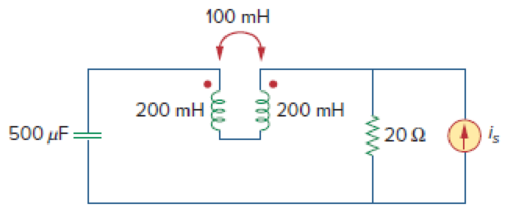
(a)
Calculate the coupling coefficient of the circuit in Figure 13.93.
Answer to Problem 24P
The coupling coefficient is
Explanation of Solution
Given data:
Refer to Figure 13.93 in the textbook for the circuit with coupled coils.
The value of
Calculation:
Consider the expression for the coefficient of coupling in the coupled coils.
Substitute 1 H for M, 4 H for
Conclusion:
Thus, the coupling coefficient is
(b)
Calculate the voltage
Answer to Problem 24P
The value of voltage
Explanation of Solution
Given data:
From Figure 13.93, the value of
Calculation:
Write the expression for the inductive reactance.
Write the expression for the capacitive reactance.
Substitute 4 H for
Substitute 2 H for
Substitute 1 H for
Substitute
Calculate load impedance
Modify the Figure 13.93 by transforming the time-domain circuit with coupled-coils to frequency domain of the circuit with coupled-coils. The frequency domain equivalent circuit is shown in Figure 1.
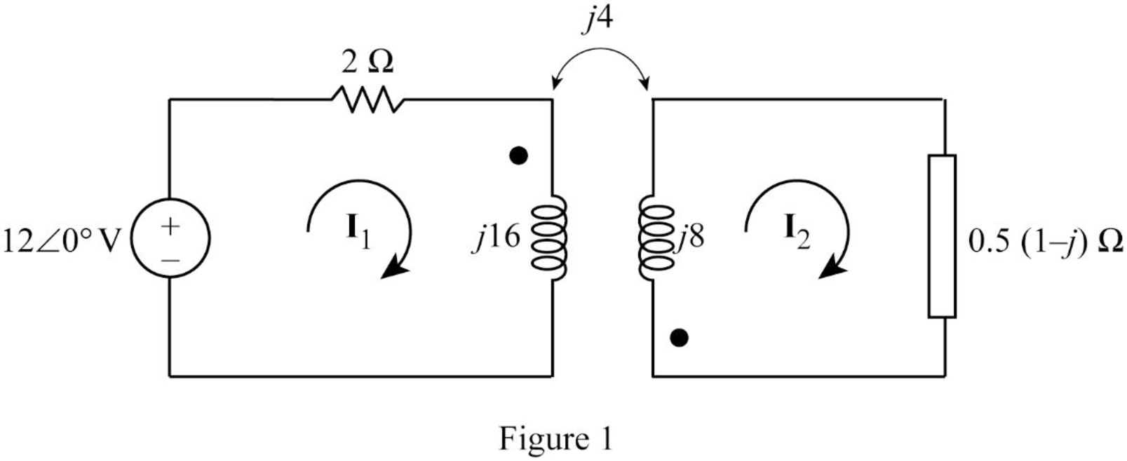
From Figure 1, consider that the loops 1 and 2 contain the currents
Apply Kirchhoff's voltage law to the loop 1 in Figure 1.
Apply Kirchhoff's voltage law to the loop 2 in Figure 1.
Write equations (3) and (4) in matrix form as follows.
Write the MATLAB code to solve the equation (5).
A = [(1+j*8) j*2;j*4 (0.5+j*7.5)];
B = [6; 0];
I = inv(A)*B
The output in command window:
I =
0.13036 - 0.84468i
-0.09912 + 0.44389i
From the MATLAB output, the currents
And
Write the expression for the voltage
Substitute
Convert the phasor form to time domain form.
Conclusion:
Thus, the value of voltage
(c)
Calculate the stored energy in the coupled coils at
Answer to Problem 24P
The energy stored in the coupled coils is
Explanation of Solution
Calculation:
From part (b), write the currents
Substitute 2 s for t in Equation (6).
Substitute 2 s for t in Equation (7).
Write the expression for the total energy stored in the coupled coils.
Substitute 4 H for
Conclusion:
Thus, the energy stored in the coupled coils is
Want to see more full solutions like this?
Chapter 13 Solutions
EBK FUNDAMENTALS OF ELECTRIC CIRCUITS
Additional Engineering Textbook Solutions
Thinking Like an Engineer: An Active Learning Approach (4th Edition)
Starting Out With Visual Basic (8th Edition)
Mechanics of Materials (10th Edition)
Starting Out with Programming Logic and Design (5th Edition) (What's New in Computer Science)
Thermodynamics: An Engineering Approach
Elementary Surveying: An Introduction To Geomatics (15th Edition)

- Find Va and Vb using nodal analysisarrow_forward2. Using the approximate method, hand sketch the Bode plot for the following transfer functions. a) H(s) = 10 b) H(s) (s+1) c) H(s): = 1 = +1 100 1000 (s+1) 10(s+1) d) H(s) = (s+100) (180+1)arrow_forwardQ4: Write VHDL code to implement the finite-state machine described by the state Diagram in Fig. 1. Fig. 1arrow_forward
- 1. Consider the following feedback system. Bode plot of G(s) is shown below. Phase (deg) Magnitude (dB) -50 -100 -150 -200 0 -90 -180 -270 101 System: sys Frequency (rad/s): 0.117 Magnitude (dB): -74 10° K G(s) Bode Diagram System: sys Frequency (rad/s): 36.8 Magnitude (dB): -99.7 System: sys Frequency (rad/s): 20 Magnitude (dB): -89.9 System: sys Frequency (rad/s): 20 Phase (deg): -143 System: sys Frequency (rad/s): 36.8 Phase (deg): -180 101 Frequency (rad/s) a) Determine the range of K for which the closed-loop system is stable. 102 10³ b) If we want the gain margin to be exactly 50 dB, what is value for K we should choose? c) If we want the phase margin to be exactly 37°, what is value of K we should choose? What will be the corresponding rise time (T) for step-input? d) If we want steady-state error of step input to be 0.6, what is value of K we should choose?arrow_forward: Write VHDL code to implement the finite-state machine/described by the state Diagram in Fig. 4. X=1 X=0 solo X=1 X=0 $1/1 X=0 X=1 X=1 52/2 $3/3 X=1 Fig. 4 X=1 X=1 56/6 $5/5 X=1 54/4 X=0 X-O X=O 5=0 57/7arrow_forwardQuestions: Q1: Verify that the average power generated equals the average power absorbed using the simulated values in Table 7-2. Q2: Verify that the reactive power generated equals the reactive power absorbed using the simulated values in Table 7-2. Q3: Why it is important to correct the power factor of a load? Q4: Find the ideal value of the capacitor theoretically that will result in unity power factor. Vs pp (V) VRIPP (V) VRLC PP (V) AT (μs) T (us) 8° pf Simulated 14 8.523 7.84 84.850 1000 29.88 0.866 Measured 14 8.523 7.854 82.94 1000 29.85 0.86733 Table 7-2 Power Calculations Pvs (mW) Qvs (mVAR) PRI (MW) Pay (mW) Qt (mVAR) Qc (mYAR) Simulated -12.93 -7.428 9.081 3.855 12.27 -4.84 Calculated -12.936 -7.434 9.083 3.856 12.32 -4.85 Part II: Power Factor Correction Table 7-3 Power Factor Correction AT (us) 0° pf Simulated 0 0 1 Measured 0 0 1arrow_forward
- Questions: Q1: Verify that the average power generated equals the average power absorbed using the simulated values in Table 7-2. Q2: Verify that the reactive power generated equals the reactive power absorbed using the simulated values in Table 7-2. Q3: Why it is important to correct the power factor of a load? Q4: Find the ideal value of the capacitor theoretically that will result in unity power factor. Vs pp (V) VRIPP (V) VRLC PP (V) AT (μs) T (us) 8° pf Simulated 14 8.523 7.84 84.850 1000 29.88 0.866 Measured 14 8.523 7.854 82.94 1000 29.85 0.86733 Table 7-2 Power Calculations Pvs (mW) Qvs (mVAR) PRI (MW) Pay (mW) Qt (mVAR) Qc (mYAR) Simulated -12.93 -7.428 9.081 3.855 12.27 -4.84 Calculated -12.936 -7.434 9.083 3.856 12.32 -4.85 Part II: Power Factor Correction Table 7-3 Power Factor Correction AT (us) 0° pf Simulated 0 0 1 Measured 0 0 1arrow_forwardelectric plants. Prepare the load schedulearrow_forwardelectric plants Draw the column diagram. Calculate the voltage drop. by hand writingarrow_forward
- electric plants. Draw the lighting, socket, telephone, TV, and doorbell installations on the given single-story project with an architectural plan by hand writingarrow_forwardA circularly polarized wave, traveling in the +z-direction, is received by an elliptically polarized antenna whose reception characteristics near the main lobe are given approx- imately by E„ = [2â, + jâ‚]ƒ(r. 8, 4) Find the polarization loss factor PLF (dimensionless and in dB) when the incident wave is (a) right-hand (CW) An elliptically polarized wave traveling in the negative z-direction is received by a circularly polarized antenna. The vector describing the polarization of the incident wave is given by Ei= 2ax + jay.Find the polarization loss factor PLF (dimensionless and in dB) when the wave that would be transmitted by the antenna is (a) right-hand CParrow_forwardjX(1)=j0.2p.u. jXa(2)=j0.15p.u. jxa(0)=0.15 p.u. V₁=1/0°p.u. V₂=1/0° p.u. 1 jXr(1) = j0.15 p.11. jXT(2) = j0.15 p.u. jXr(0) = j0.15 p.u. V3=1/0° p.u. А V4=1/0° p.u. 2 jX1(1)=j0.12 p.u. 3 jX2(1)=j0.15 p.u. 4 jX1(2)=0.12 p.11. JX1(0)=0.3 p.u. jX/2(2)=j0.15 p.11. X2(0)=/0.25 p.1. Figure 1. Circuit for Q3 b).arrow_forward
 Delmar's Standard Textbook Of ElectricityElectrical EngineeringISBN:9781337900348Author:Stephen L. HermanPublisher:Cengage Learning