Concept explainers
Videos
a)
To determine: The optimal plan using the transportation method.
Introduction: Aggregate planning using transportation method helps to attain minimum cost using the optimal plan. The major advantage of transportation method is to achieve the optimal solution using optimal plans.
a)
Answer to Problem 17P
The optimal plan using the transportation method has been developed.
Explanation of Solution
Given information:
The following information has been given:
| Quarter |
| Regular time | Overtime | Subcontract |
| 1 | 500 | 400 | 80 | 100 |
| 2 | 750 | 400 | 80 | 100 |
| 3 | 900 | 800 | 160 | 100 |
| 4 | 450 | 400 | 80 | 100 |
Initial inventory is given as 250 units, regular time cost is $1 per unit, overtime cost is $1.50 per unit, and subcontract cost is $2 per unit. Carrying cost is given as $0.5 per unit per quarter and backorder cost is $0.5 per unit per quarter. Initial inventory would incur $0.2 per unit.
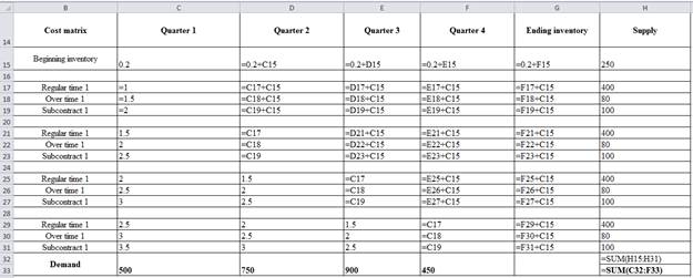
Develop optimal plan using transportation model:
Develop cost matrix:
| Cost matrix | Quarter 1 | Quarter 2 | Quarter 3 | Quarter 4 | Ending inventory | Supply |
| Beginning inventory | 0.2 | 0.4 | 0.6 | 0.8 | 1 | 250 |
| Regular time 1 | 1 | 1.2 | 1.4 | 1.6 | 1.8 | 400 |
| Over time 1 | 1.5 | 1.7 | 1.9 | 2.1 | 2.3 | 80 |
| Subcontract 1 | 2 | 2.2 | 2.4 | 2.6 | 2.8 | 100 |
| Regular time 1 | 1.5 | 1 | 1.2 | 1.4 | 1.6 | 400 |
| Over time 1 | 2 | 1.5 | 1.7 | 1.9 | 2.1 | 80 |
| Subcontract 1 | 2.5 | 2 | 2.2 | 2.4 | 2.6 | 100 |
| Regular time 1 | 2 | 1.5 | 1 | 1.2 | 1.4 | 400 |
| Over time 1 | 2.5 | 2 | 1.5 | 1.7 | 1.9 | 80 |
| Subcontract 1 | 3 | 2.5 | 2 | 2.2 | 2.4 | 100 |
| Regular time 1 | 2.5 | 2 | 1.5 | 1 | 1.2 | 400 |
| Over time 1 | 3 | 2.5 | 2 | 1.5 | 1.7 | 80 |
| Subcontract 1 | 3.5 | 3 | 2.5 | 2 | 2.2 | 100 |
| Demand | 500 | 750 | 900 | 450 | 2570 | |
| 2600 |
Excel worksheet to generate the above table:
Develop optimal plan:
| Optimal plan | Quarter 1 | Quarter 2 | Quarter 3 | Quarter 4 | Ending inventory | Dummy |
| Beginning inventory | 100 | 150 | ||||
| Regular time 1 | 400 | |||||
| Over time 1 | 80 | |||||
| Subcontract 1 | 100 | |||||
| Regular time 1 | 400 | |||||
| Over time 1 | 80 | |||||
| Subcontract 1 | 100 | |||||
| Regular time 1 | 800 | |||||
| Over time 1 | 40 | 100 | 20 | |||
| Subcontract 1 | 100 | |||||
| Regular time 1 | 400 | |||||
| Over time 1 | 50 | 30 | ||||
| Subcontract 1 | 100 | |||||
| Demand | 500 | 750 | 900 | 450 |
The given demand and supply should be separated and the remaining supply and demand should be used as a dummy value.
b)
To determine: The total cost of the optimal plan.
Introduction: Aggregate planning using transportation method helps to attain minimum cost using the optimal plan. The major advantage of transportation method is to achieve the optimal solution using optimal plans.
b)
Answer to Problem 17P
The optimal cost of the plan is $2,641.
Explanation of Solution
Given information:
The following information has been given:
| Quarter | Forecast (units) | Regular time | Overtime | Subcontract |
| 1 | 500 | 400 | 80 | 100 |
| 2 | 750 | 400 | 80 | 100 |
| 3 | 900 | 800 | 160 | 100 |
| 4 | 450 | 400 | 80 | 100 |
Initial inventory is given as 250 units, regular time cost is $1 per unit, overtime cost is $1.50 per unit, and subcontract cost is $2 per unit. Carrying cost is given as $0.5 per unit per quarter and backorder cost is $0.5 per unit per quarter. Initial inventory would incur $0.2 per unit.
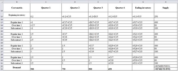
Develop optimal plan using transportation model:
Develop cost matrix:
| Cost matrix | Quarter 1 | Quarter 2 | Quarter 3 | Quarter 4 | Ending inventory | Supply |
| Beginning inventory | 0.2 | 0.4 | 0.6 | 0.8 | 1 | 250 |
| Regular time 1 | 1 | 1.2 | 1.4 | 1.6 | 1.8 | 400 |
| Over time 1 | 1.5 | 1.7 | 1.9 | 2.1 | 2.3 | 80 |
| Subcontract 1 | 2 | 2.2 | 2.4 | 2.6 | 2.8 | 100 |
| Regular time 1 | 1.5 | 1 | 1.2 | 1.4 | 1.6 | 400 |
| Over time 1 | 2 | 1.5 | 1.7 | 1.9 | 2.1 | 80 |
| Subcontract 1 | 2.5 | 2 | 2.2 | 2.4 | 2.6 | 100 |
| Regular time 1 | 2 | 1.5 | 1 | 1.2 | 1.4 | 400 |
| Over time 1 | 2.5 | 2 | 1.5 | 1.7 | 1.9 | 80 |
| Subcontract 1 | 3 | 2.5 | 2 | 2.2 | 2.4 | 100 |
| Regular time 1 | 2.5 | 2 | 1.5 | 1 | 1.2 | 400 |
| Over time 1 | 3 | 2.5 | 2 | 1.5 | 1.7 | 80 |
| Subcontract 1 | 3.5 | 3 | 2.5 | 2 | 2.2 | 100 |
| Demand | 500 | 750 | 900 | 450 | 2570 | |
| 2600 |
Excel worksheet to generate the above table:
Develop optimal plan:
| Optimal plan | Quarter 1 | Quarter 2 | Quarter 3 | Quarter 4 | Ending inventory | Dummy |
| Beginning inventory | 100 | 150 | ||||
| Regular time 1 | 400 | |||||
| Over time 1 | 80 | |||||
| Subcontract 1 | 100 | |||||
| Regular time 1 | 400 | |||||
| Over time 1 | 80 | |||||
| Subcontract 1 | 100 | |||||
| Regular time 1 | 800 | |||||
| Over time 1 | 40 | 100 | 20 | |||
| Subcontract 1 | 100 | |||||
| Regular time 1 | 400 | |||||
| Over time 1 | 50 | 30 | ||||
| Subcontract 1 | 100 | |||||
| Demand | 500 | 750 | 900 | 450 |
The given demand and supply should be splitted and the remaining supply and demand should be used as a dummy value.
Calculate the total optimal cost:
It is calculated by adding the multiple of values in the optimal plan table and the value in the cost matrix to the respective value.
Hence, the total optimal cost is $2,641.
c)
To determine: The number of units remained unused in regular time capacity.
Introduction: Aggregate planning using transportation method helps to attain minimum cost using the optimal plan. The major advantage of transportation method is to achieve the optimal solution using optimal plans.
c)
Answer to Problem 17P
No, the regular time capacity remains unused.
Explanation of Solution
Given information:
The following information has been given:
| Quarter | Forecast (units) | Regular time | Overtime | Subcontract |
| 1 | 500 | 400 | 80 | 100 |
| 2 | 750 | 400 | 80 | 100 |
| 3 | 900 | 800 | 160 | 100 |
| 4 | 450 | 400 | 80 | 100 |
Initial inventory is given as 250 units, regular time cost is $1 per unit, overtime cost is $1.50 per unit, and subcontract cost is $2 per unit. Carrying cost is given as $0.5 per unit per quarter and backorder cost is $0.5 per unit per quarter. Initial inventory would incur $0.2 per unit.
Develop optimal plan:
| Optimal plan | Quarter 1 | Quarter 2 | Quarter 3 | Quarter 4 | Ending inventory | Dummy |
| Beginning inventory | 100 | 150 | ||||
| Regular time 1 | 400 | |||||
| Over time 1 | 80 | |||||
| Subcontract 1 | 100 | |||||
| Regular time 1 | 400 | |||||
| Over time 1 | 80 | |||||
| Subcontract 1 | 100 | |||||
| Regular time 1 | 800 | |||||
| Over time 1 | 40 | 100 | 20 | |||
| Subcontract 1 | 100 | |||||
| Regular time 1 | 400 | |||||
| Over time 1 | 50 | 30 | ||||
| Subcontract 1 | 100 | |||||
| Demand | 500 | 750 | 900 | 450 |
The given demand and supply should be separated and the remaining supply and demand should be used as a dummy value.
Determine whether the regular time capacity remain unused:
From the above table, it is clear that no regular time capacity remains unused. All the regular time capacity has been used in respective quarters.
d)
To determine: The extent of backordering in units and dollars.
Introduction: Aggregate planning using transportation method helps to attain minimum cost using the optimal plan. The major advantage of transportation method is to achieve the optimal solution using optimal plans.
d)
Answer to Problem 17P
The total unit of the backordered is 40 units and the total cost of producing the backorders are $20.
Explanation of Solution
Given information:
The following information has been given:
| Quarter | Forecast (units) | Regular time | Overtime | Subcontract |
| 1 | 500 | 400 | 80 | 100 |
| 2 | 750 | 400 | 80 | 100 |
| 3 | 900 | 800 | 160 | 100 |
| 4 | 450 | 400 | 80 | 100 |
Initial inventory is given as 250 units, regular time cost is $1 per unit, overtime cost is $1.50 per unit, and subcontract cost is $2 per unit. Carrying cost is given as $0.5 per unit per quarter and backorder cost is $0.5 per unit per quarter. Initial inventory would incur $0.2 per unit.
Develop optimal plan:
| Optimal plan | Quarter 1 | Quarter 2 | Quarter 3 | Quarter 4 | Ending inventory | Dummy |
| Beginning inventory | 100 | 150 | ||||
| Regular time 1 | 400 | |||||
| Over time 1 | 80 | |||||
| Subcontract 1 | 100 | |||||
| Regular time 1 | 400 | |||||
| Over time 1 | 80 | |||||
| Subcontract 1 | 100 | |||||
| Regular time 1 | 800 | |||||
| Over time 1 | 40 | 100 | 20 | |||
| Subcontract 1 | 100 | |||||
| Regular time 1 | 400 | |||||
| Over time 1 | 50 | 30 | ||||
| Subcontract 1 | 100 | |||||
| Demand | 500 | 750 | 900 | 450 |
The given demand and supply should be separated and the remaining supply and demand should be used as a dummy value.
Determine the extent backordering in units and dollars:
The colored cell is the only cell in the optimal plan, which is used for backordering. Hence, the backordering in units is 40 units. It is given that backorder cost is $0.50 per unit per quarter.
Hence, the total unit backordered is 40 units and the total costs of producing the backorders are $20.
Want to see more full solutions like this?
Chapter 13 Solutions
EBK PRINCIPLES OF OPERATIONS MANAGEMENT


- Prepare a graph of the monthly forecasts and average forecast demand for Chicago Paint Corp., a manufacturer of specialized paint for artists. Compute the demand per day for each month (round your responses to one decimal place). Month B Production Days Demand Forecast Demand per Day January 21 950 February 19 1,150 March 21 1,150 April 20 1,250 May 23 1,200 June 22 1,000' July 20 1,350 August 21 1,250 September 21 1,050 October 21 1,050 November 21 December 225 950 19 850arrow_forwardThe president of Hill Enterprises, Terri Hill, projects the firm's aggregate demand requirements over the next 8 months as follows: 2,300 January 1,500 May February 1,700 June 2,100 March April 1,700 1,700 July August 1,900 1,500 Her operations manager is considering a new plan, which begins in January with 200 units of inventory on hand. Stockout cost of lost sales is $125 per unit. Inventory holding cost is $25 per unit per month. Ignore any idle-time costs. The plan is called plan C. Plan C: Keep a stable workforce by maintaining a constant production rate equal to the average gross requirements excluding initial inventory and allow varying inventory levels. Conduct your analysis for January through August. The average monthly demand requirement = units. (Enter your response as a whole number.) In order to arrive at the costs, first compute the ending inventory and stockout units for each month by filling in the table below (enter your responses as whole numbers). Ending E Period…arrow_forwardMention four early warning indicators that a business may be at risk.arrow_forward
- 1. Define risk management and explain its importance in a small business. 2. Describe three types of risks commonly faced by entrepreneurs. 3. Explain the purpose of a risk register. 4. List and briefly describe four risk response strategies. (5 marks) (6 marks) (4 marks) (8 marks) 5. Explain how social media can pose a risk to small businesses. (5 marks) 6. Identify and describe any four hazard-based risks. (8 marks) 7. Mention four early warning indicators that a business may be at risk. (4 marks)arrow_forwardState whether each of the following statements is TRUE or FALSE. 1. Risk management involves identifying, analysing, and mitigating risks. 2. Hazard risks include interest rate fluctuations. 3. Entrepreneurs should avoid all forms of risks. 4. SWOT analysis is a tool for risk identification. 5. Scenario building helps visualise risk responses. 6. Risk appetite defines how much risk an organisation is willing to accept. 7. Diversification is a risk reduction strategy. 8. A risk management framework must align with business goals. 9. Political risk is only relevant in unstable countries. 10. All risks can be eliminated through insurance.arrow_forward9. A hazard-based risk includes A. Political instability B. Ergonomic issues C. Market demand D. Taxation changesarrow_forward

 Purchasing and Supply Chain ManagementOperations ManagementISBN:9781285869681Author:Robert M. Monczka, Robert B. Handfield, Larry C. Giunipero, James L. PattersonPublisher:Cengage Learning
 Practical Management ScienceOperations ManagementISBN:9781337406659Author:WINSTON, Wayne L.Publisher:Cengage,
- MarketingMarketingISBN:9780357033791Author:Pride, William MPublisher:South Western Educational Publishing