Concept explainers
Licensed drivers. Table 9 contains the state population and the number of licensed drivers in the state (both in millions) for the most populous states in 2014. The regression model for this data is
where
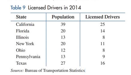
(A) Draw a
(B) If the population of Michigan in 2014 was about 9.9 million, use the model to estimate
the number of licensed drivers in Michigan in 2014 to the nearest thousand.
(C) If the number of licensed drivers in Georgia in 2014 was about 6.7 million, use the model
to estimate the population of Georgia in 2014 to the nearest thousand.
Want to see the full answer?
Check out a sample textbook solution
Chapter 1 Solutions
Finite Mathematics for Business, Economics, Life Sciences and Social Sciences
Additional Math Textbook Solutions
College Algebra (7th Edition)
Thinking Mathematically (6th Edition)
Pre-Algebra Student Edition
Calculus: Early Transcendentals (2nd Edition)
A Problem Solving Approach To Mathematics For Elementary School Teachers (13th Edition)
- A ball is thrown into the air and its height (in meters) is given by h (t) in seconds. -4.92 + 30t+1, where t is a. After how long does the ball reach its maximum height? Round to 2 decimal places. seconds b. What is the maximum height of the ball? Round to 2 decimal places. metersarrow_forwardDetermine where the absolute and local extrema occur on the graph given. Assume the domain is a closed interval and the graph represents the entirety of the function. 1.5 y 1 0.5 -3 -2 -0.5 -1 -1.5 Separate multiple answers with a comma. Absolute maximum at Absolute minimum at Local maxima at Local minima at a x 2 3 аarrow_forwardA company that produces cell phones has a cost function of C = x² - 1000x + 36100, where C is the cost in dollars and x is the number of cell phones produced (in thousands). How many units of cell phones (in thousands) minimizes this cost function? Round to the nearest whole number, if necessary. thousandarrow_forward
- 11:48 SS retry this question below lll 43% A communications tower is located at the top of a steep hill, as shown. The angle of inclination of the hill is 77°. A guy wire is to be attached to the top of the tower and to the ground, 102 ft downhill from the base of the tower. The angle formed by the guy wire is 9°. Find the length of the cable required for the guy wire. 9° 102 ft 77° NOTE: The picture is NOT drawn to scale. length of guy-wire = ft Enter your answer as a number; your answer should be accurate to 2 decimal places. Question Help: Video Submit Question Jump to Answer |||arrow_forwardHow come that I marked ?arrow_forwardUnder certain conditions, the number of diseased cells N(t) at time t increases at a rate N'(t) = Aekt, where A is the rate of increase at time 0 (in cells per day) and k is a constant. (a) Suppose A = 60, and at 3 days, the cells are growing at a rate of 180 per day. Find a formula for the number of cells after t days, given that 200 cells are present at t = 0. (b) Use your answer from part (a) to find the number of cells present after 8 days. (a) Find a formula for the number of cells, N(t), after t days. N(t) = (Round any numbers in exponents to five decimal places. Round all other numbers to the nearest tenth.)arrow_forward
- The marginal revenue (in thousands of dollars) from the sale of x handheld gaming devices is given by the following function. R'(x) = 4x (x² +26,000) 2 3 (a) Find the total revenue function if the revenue from 125 devices is $17,939. (b) How many devices must be sold for a revenue of at least $50,000? (a) The total revenue function is R(x) = (Round to the nearest integer as needed.) given that the revenue from 125 devices is $17,939.arrow_forwardUse substitution to find the indefinite integral. S 2u √u-4 -du Describe the most appropriate substitution case and the values of u and du. Select the correct choice below and fill in the answer boxes within your choice. A. Substitute u for the quantity in the numerator. Let v = , so that dv = ( ) du. B. Substitute u for the quantity under the root. Let v = u-4, so that dv = (1) du. C. Substitute u for the quantity in the denominator. Let v = Use the substitution to evaluate the integral. so that dv= ' ( du. 2u -du= √√u-4arrow_forwardConsider the state space model X₁ = §Xt−1 + Wt, Yt = AX+Vt, where Xt Є R4 and Y E R². Suppose we know the covariance matrices for Wt and Vt. How many unknown parameters are there in the model?arrow_forward
- Use substitution to find the indefinite integral. Зи u-8 du Describe the most appropriate substitution case and the values of u and du. Select the correct choice below and fill in the answer boxes within your choice. A. Substitute u for the quantity in the numerator. Let v = , so that dv = ( ( ) du. B. Substitute u for the quantity under the root. Let v = u-8, so that dv = (1) du. C. Substitute u for the quantity in the denominator. Let v = so that dv= ( ) du. Use the substitution to evaluate the integral. S Зи -du= u-8arrow_forwardAloha Airlines Flight 007 is flying due east but finds it necessary to detour around a group of thundershowers. The plane 1st turns at a bearing of N 73° E, flies for a while, then 2nd turns to intercept the original path and travels for 50 km at a bearing of S 41° E, back to the original path. As stated the plane traveled 50 km in the 2nd leg of the journey getting back to the path. How far did the plane travel in the 1st leg of the journey?arrow_forwardQuestion 6 Aloha Airlines Flight 007 is flying due east but finds it necessary to detour around a group of thundershowers. The plane 1st turns at a bearing of N 73° E, flies for a while, then 2nd turns to intercept the original path and travels for 50 km at a bearing of S 41° E, back to the original path. As stated the plane traveled 50 km in the 2nd leg of the journey getting back to the path. How far did the plane travel in the 1st leg of the journey? Question Help: Video Submit Question Jump to Answer P3 E E T Q Search L W F1 % R R FS F € t X C V 08 7 47 * B FB Y I E 7 コ コ I Barrow_forward

 Glencoe Algebra 1, Student Edition, 9780079039897...AlgebraISBN:9780079039897Author:CarterPublisher:McGraw Hill
 Functions and Change: A Modeling Approach to Coll...AlgebraISBN:9781337111348Author:Bruce Crauder, Benny Evans, Alan NoellPublisher:Cengage Learning
 Elementary Linear Algebra (MindTap Course List)AlgebraISBN:9781305658004Author:Ron LarsonPublisher:Cengage Learning
 Holt Mcdougal Larson Pre-algebra: Student Edition...AlgebraISBN:9780547587776Author:HOLT MCDOUGALPublisher:HOLT MCDOUGAL


