Chapter 12, Problem 6P

(a)

To determine

Draw the influence lines for the reactions $B,C,E,\text{and}G$ of the beam and moments at $C$ and E.

Determine the reactions at B, C, D and E, moments at C and D.

Explanation of Solution

Given Information:

The uniform load (w) is 2 kips/ft.

Calculation:

Influence line for reaction at $G$.

Consider the portion AF $\left(0\le x<80\text{ft}\right)$.

Apply a 1 kip unit moving load at a distance of $x$ from A in the portion AF.

Sketch the free body diagram of beam as shown in Figure 1.

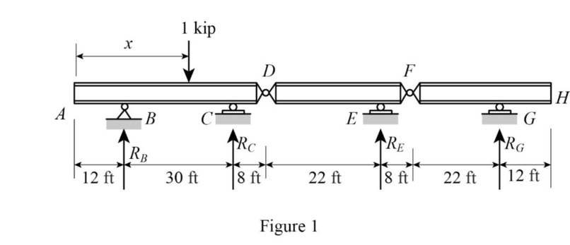
Refer Figure 1.

Find the equation support reaction $\left(R_G\right)$.

Take moment about point F from H.

Consider clockwise moment as negative and anticlockwise moment as positive

$\begin{array}{l}\Sigma M_F=0\\ R_G\left(22\right)=0\\ R_G=0\end{array}$

Consider the portion FH $\left(80\text{ft}<x\le 114\text{ft}\right)$.

Apply a 1 kip unit moving load at a distance of $x$ from A in the portion GH.

Sketch the free body diagram of beam as shown in Figure 2.

Refer Figure 2.

Consider clockwise moment as negative and anticlockwise moment as positive.

Find the equation support reaction $\left(R_G\right)$.

Take moment about point F from H.

$\begin{array}{l}\Sigma M_F=0\\ R_G\left(22\right)-1\left(x-80\right)=0\\ R_G=\frac{x-80}{22}\end{array}$

Thus, the equations of the influence line for $R_G$ are,

$R_G=00\le x\le 80\text{ft}$        (1)

$R_G=\frac{x-80}{22}80\text{ft}\le x\le 114\text{ft}$        (2)

Find the value of influence line ordinate of $R_G$ for various points of x using the Equations (1) and (2) and summarize the value as in Table 1.

Points	x $\left(\text{ft}\right)$	$R_G$
A	0	0
$B$	12	0
C	42	0
D	50	0
E	72	0
F	80	0
G	102	1
H	114	1.55

Draw the influence lines for $R_G$ using Table 1 as shown in Figure 3.

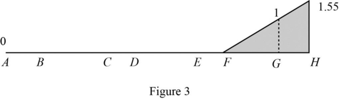
Refer Figure 3.

Determine the reaction at G.

$\begin{array}{c}{R}_G=\frac{1}{2}\left(1.55\right)\left(114-80\right)\left(w\right)\\ =\frac{1}{2}\left(1.55\right)\left(34\right)\left(2\right)\\ =52.7\text{k}\end{array}$

Therefore, the reaction at G is $\underset{\_}{52.7\text{k}}$

Influence line for reaction $R_E$.

Consider the portion AD $\left(0\le x\le 50\text{ft}\right)$.

Apply a 1 kip unit moving load at a distance of $x$ from A in the portion AD.

Sketch the free body diagram of beam as shown in Figure 4.

Refer Figure 4.

Find the equation support reaction $\left(R_E\right)$.

Take moment about point D from H.

Consider clockwise moment as negative and anticlockwise moment as positive

$\begin{array}{l}\Sigma M_D=0\\ R_G\left(52\right)+R_E\left(22\right)=0\\ \left(0\right)\left(52\right)+R_E\left(22\right)=0\\ R_E=0\end{array}$

Consider the portion DF $\left(50\text{ft}\le x\le 80\text{ft}\right)$.

Apply a 1 kip unit moving load at a distance of $x$ from A in the portion DF.

Sketch the free body diagram of beam as shown in Figure 5.

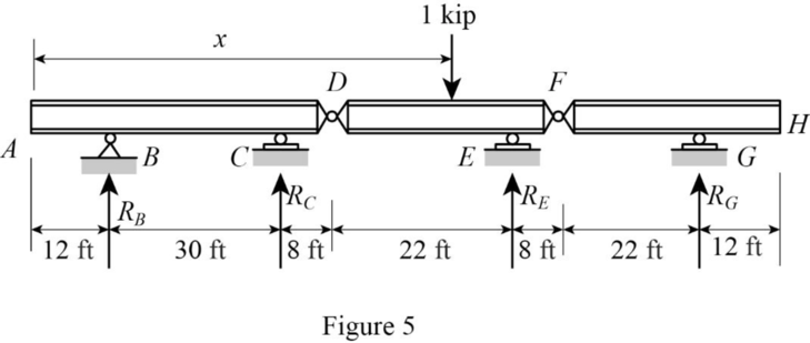
Refer Figure 5.

Find the equation support reaction $\left(R_E\right)$.

Take moment about point F from H.

$\begin{array}{l}\Sigma M_D=0\\ R_G\left(52\right)+R_E\left(22\right)-1\left(x-50\right)=0\\ \left(0\right)\left(52\right)+R_E\left(22\right)=x-50\\ R_E=\frac{x-50}{22}\end{array}$

Consider the portion FH $\left(80\text{ft}\le x\le 114\text{ft}\right)$.

Apply a 1 kip unit moving load at a distance of $x$ from A in the portion FH.

Sketch the free body diagram of beam as shown in Figure 6.

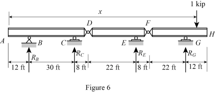
Refer Figure 6.

Find the equation support reaction $\left(R_E\right)$.

Take moment about point F from H.

$\begin{array}{l}\Sigma M_D=0\\ R_G\left(52\right)+R_E\left(22\right)-1\left(x-50\right)=0\\ \left(\frac{x-80}{22}\right)\left(52\right)+R_E\left(22\right)=x-50\\ 2.364x-189.1+22R_E=x-50\end{array}$

$\begin{array}{l}22R_E=x-50-2.364x+189.1\\ 22R_E=139.1-1.364x\\ R_E=6.323-0.062x\end{array}$

Thus, the equations of the influence line for $R_E$ are,

$R_E=00\le x\le 50\text{ft}$        (3)

$R_E=\frac{x-50}{22}50\text{ft}\le x\le 80\text{ft}$        (4)

$R_E=6.323-0.062x80\text{ft}\le x\le 114\text{ft}$        (5)

Find the value of influence line ordinate of $R_E$ for various points of x using the Equations (1) and (2) and summarize the value as in Table 2.

Points	x $\left(\text{ft}\right)$	$R_E$
A	0	0
$B$	12	0
C	42	0
D	50	0
E	72	1
F	80	1.364
G	102	0
H	114	‑0.744

Draw the influence lines for $R_E$ using Table 2 as shown in Figure 7.

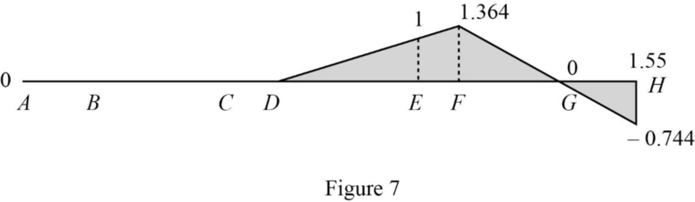
Refer Figure 7.

Determine the reaction at E.

$\begin{array}{c}{R}_E=\frac{1}{2}\left(1.364\right)\left(102-50\right)\left(w\right)+\frac{1}{2}\left(-0.744\right)\left(114-112\right)\left(w\right)\\ =\frac{1}{2}\left(1.364\right)\left(102-50\right)\left(2\right)+\frac{1}{2}\left(-0.744\right)\left(114-102\right)\left(2\right)\\ =70.928-8.928\\ =62\text{k}\end{array}$

Therefore, the reaction at E is $\underset{\_}{62\text{k}}$

Influence line for reaction $R_C$.

Consider the portion AD $\left(0\le x\le 50\text{ft}\right)$.

Apply a 1 kip unit moving load at a distance of $x$ from A in the portion AB.

Sketch the free body diagram of beam as shown in Figure 8.

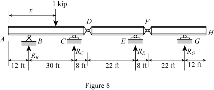
Refer Figure 8.

Find the equation support reaction $\left(R_C\right)$.

Take moment about point B from H.

$\begin{array}{l}\Sigma M_B=0\\ R_G\left(70\right)+R_E\left(60\right)-1\left(x-12\right)+R_C\left(30\right)=0\\ \left(0\right)\left(90\right)+\left(0\right)\left(60\right)-x+12+30R_C=0\\ 30R_C=x-12\\ R_C=0.033x-0.4\end{array}$

Consider the portion DF $\left(50\text{ft}\le x\le 80\text{ft}\right)$.

Apply a 1 kip unit moving load at a distance of $x$ from A in the portion DF.

Sketch the free body diagram of beam as shown in Figure 9.

Refer Figure 9.

Find the equation support reaction $\left(R_E\right)$.

Take moment about point B from H.

$\begin{array}{l}\Sigma M_B=0\\ R_G\left(90\right)+R_E\left(60\right)-1\left(x-12\right)+R_C\left(30\right)=0\\ \left(0\right)\left(90\right)+\left(\frac{x-50}{22}\right)\left(60\right)-x+12+30R_C=0\\ \frac{60x-3,000}{22}-x+12+30R_C=0\\ 30R_C=124.364-1.727x\\ R_C=4.15-0.0576x\end{array}$

Consider the portion FH $\left(80\text{ft}\le x\le 114\text{ft}\right)$.

Apply a 1 kip unit moving load at a distance of $x$ from A in the portion FH.

Sketch the free body diagram of beam as shown in Figure 10.

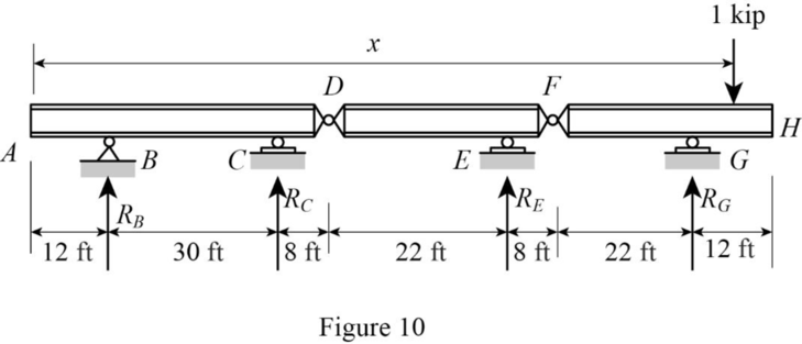
Refer Figure 6.

Find the equation support reaction $\left(R_D\right)$.

Take moment about point B from H.

Consider clockwise moment as negative and anticlockwise moment as positive

$\begin{array}{l}\Sigma M_B=0\\ R_G\left(90\right)+R_E\left(60\right)-1\left(x-12\right)+R_C\left(30\right)=0\\ \left(\frac{x-80}{22}\right)\left(90\right)+\left(6.323-0.062x\right)\left(60\right)-x+12+30R_C=0\\ 4.1x-327.27+379.38-3.72x-x+12+30R_C=0\\ -0.62x+64.11+30R_C=0\\ R_C=0.021x-2.14\end{array}$

Thus, the equations of the influence line for $R_E$ are,

$R_C=0.033x-0.40\le x\le 50\text{ft}$        (6)

$R_C=4.15-0.0576x50\text{ft}\le x\le 80\text{ft}$        (7)

$R_C=0.021x-2.1480\text{ft}\le x\le 114\text{ft}$        (8)

Find the value of influence line ordinate of $R_C$ for various points of x using the Equations (6), (7) and (8) and summarize the value as in Table 3.

Points	x $\left(\text{ft}\right)$	$R_C$
A	0	‑0.4
$B$	12	0
C	42	1
D	50	1.27
E	72	0
F	80	‑0.46
G	102	0
H	114	0.25

Draw the influence lines for $R_C$ using Table 3 as shown in Figure 11.

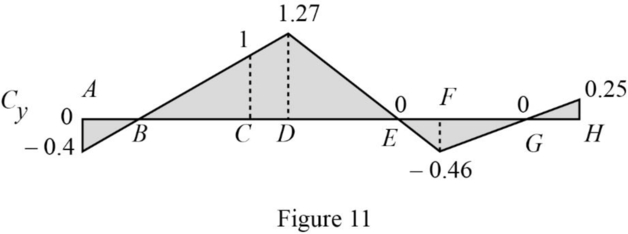
Refer Figure 11.

Determine the reaction at C.

$\begin{array}{c}{R}_C=w\left[\begin{array}{l}\frac{1}{2}\left(-0.4\right)\left(12-0\right)+\frac{1}{2}\left(1.27\right)\left(72-12\right)\\ +\frac{1}{2}\left(-0.46\right)\left(102-72\right)+\frac{1}{2}\left(0.25\right)\left(114-102\right)\end{array}\right]\\ =2\left(-2.4+38.1-6.9+1.5\right)\\ =60.6\text{k}\end{array}$

Therefore, the reaction at C is $\underset{\_}{60.6\text{k}}$

Influence line for reaction $R_B$.

Consider the portion AD $\left(0\le x\le 50\text{ft}\right)$.

Refer Figure 8.

Consider upward force as positive and anticlockwise moment as negative.

Find the equation support reaction $\left(R_B\right)$.

Consider vertical equilibrium equation.

$\begin{array}{l}\Sigma F_y=0\\ R_B+R_C+R_E+R_G-1=0\\ R_B+0.033x-0.4+0+0-1=0\\ R_B=1.4-0.033x\end{array}$

Consider the portion DF $\left(50\text{ft}\le x\le 80\text{ft}\right)$.

Refer Figure 9.

Find the equation support reaction $\left(R_B\right)$.

Consider vertical equilibrium equation.

$\begin{array}{l}\Sigma F_y=0\\ R_B+R_C+R_E+R_G-1=0\\ R_B+4.15-0.0576x+\frac{x-50}{22}+0-1=0\\ R_B+4.15-0.0576x+0.0455x-2.273-1=0\\ R_B=0.012x-0.877\end{array}$

Consider the portion FH $\left(80\text{ft}\le x\le 114\text{ft}\right)$.

Refer Figure 6.

Find the equation support reaction $\left(R_B\right)$.

Consider vertical equilibrium equation.

Consider upward force as positive and anticlockwise moment as negative.

$\begin{array}{l}\Sigma F_y=0\\ R_B+R_C+R_E+R_G-1=0\\ R_B+0.021x-2.14+6.323-0.062x+\frac{x-80}{22}-1=0\\ R_B+0.021x-2.14+6.323-0.062x+0.0455x-3.636-1=0\\ R_B=0.45-0.0045x\end{array}$

Thus, the equations of the influence line for $R_B$ are,

$R_B=1.4-0.033x0\le x\le 50\text{ft}$        (9)

$R_B=0.0121x-0.87750\text{ft}\le x\le 80\text{ft}$        (10)

$R_B=0.45-0.0045x80\text{ft}\le x\le 114\text{ft}$        (11)

Find the value of influence line ordinate of $R_B$ for various points of x using the Equations (9), (10) and (11) and summarize the value as in Table 4.

Points	x $\left(\text{ft}\right)$	$R_B$
A	0	1.4
$B$	12	1
C	42	0
D	50	‑0.25
E	72	0
F	80	0.1
G	102	0
H	114	0.063

Draw the influence lines for $R_B$ using Table 4 as shown in Figure 12.

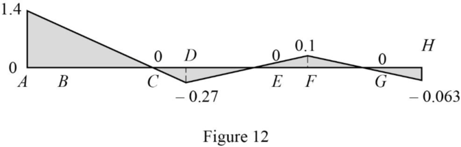
Refer Figure 12.

Determine the reaction at B.

$\begin{array}{c}{R}_B=w\left[\begin{array}{l}\frac{1}{2}\left(1.4\right)\left(42-0\right)+\frac{1}{2}\left(-0.27\right)\left(72-42\right)\\ +\frac{1}{2}\left(0.1\right)\left(102-72\right)+\frac{1}{2}\left(-0.063\right)\left(114-102\right)\end{array}\right]\\ =2\left(29.4-4.05+1.5-0.378\right)\\ =53\text{k}\end{array}$

Therefore, the reaction at B is $\underset{\_}{53\text{k}}$.

Influence line for the moment at section C:

Consider portion AC $\left(0\le x<42\text{m}\right)$

Find the equation of moment at C for portion AC.

Apply a 1 kip in the portion AC from A.

Sketch the free body diagram of the section CH as shown in Figure 13.

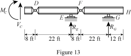
Find the equation of moment at C of portion AC.

$\begin{array}{l}{R}_G\left(60\right)+R_E\left(30\right)-M_C=0\\ M_C=\left(0\right)\left(60\right)+\left(0\right)\left(30\right)\\ M_C=0\end{array}$

Consider portion CD $\left(42<x\le 50\text{m}\right)$:

Find the equation of moment at C for portion CD.

Apply a 1 kip in the portion CD from A.

Sketch the free body diagram of the section AC as shown in Figure 14.

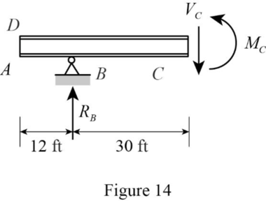
Find the equation of moment at C of portion CD.

$\begin{array}{l}-R_B\left(30\right)+M_C=0\\ M_C=\left(1.4-0.033x\right)\left(30\right)\\ M_C=42-x\end{array}$

Consider portion DF $\left(50\le x\le 80\text{m}\right)$:

Find the equation of moment at C for portion DF.

Apply a 1 kip in the portion DF from A.

Sketch the free body diagram of the section AC as shown in Figure 15.

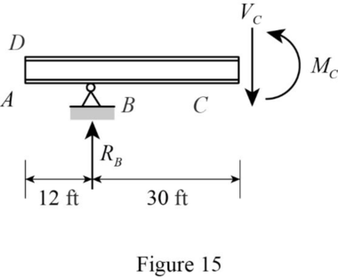
Find the equation of moment at C of portion DF.

$\begin{array}{l}-R_B\left(30\right)+M_C=0\\ M_C=\left(0.0121x-0.877\right)\left(30\right)\\ M_C=0.363x-26.31\end{array}$

Consider portion FH $\left(80\le x\le 114\text{m}\right)$:

Find the equation of moment at C for portion FH.

Apply a 1 kip in the portion FH from A.

Sketch the free body diagram of the section AC as shown in Figure 16.

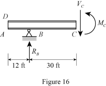
Find the equation of moment at C of portion FH.

$\begin{array}{l}-R_B\left(30\right)+M_C=0\\ M_C=\left(0.45-0.0045x\right)\left(30\right)\\ M_C=13.5-0.135x\end{array}$

Thus, the equations of the influence line for $M_C$ are,

$M_C=00\le x\le 42\text{ft}$        (12)

$M_C=42-x42\text{ft}\le x\le 50\text{ft}$        (13)

$M_C=0.363x-26.3150\text{ft}\le x\le 80\text{ft}$        (14)

$M_C=13.5-0.135x80\text{ft}\le x\le 114\text{ft}$        (15)

Find the value of influence line ordinate of $R_C$ for various points of x using the Equations (12), (13), (14) and (15) and summarize the value as in Table 5.

Points	x $\left(\text{ft}\right)$	$M_C$
A	0	0
$B$	12	0
C	42	0
D	50	‑8
E	72	0
F	80	+2.73
G	102	0
H	114	‑1.89

Draw the influence lines for $M_C$ using Table 4 as shown in Figure 17.

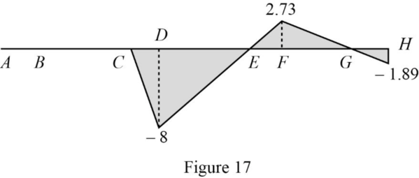
Refer Figure 17.

Determine the moment at C.

$\begin{array}{c}{M}_C=w\left[\begin{array}{l}\frac{1}{2}\left(-8\right)\left(72-42\right)+\frac{1}{2}\left(2.73\right)\left(102-72\right)\\ +\frac{1}{2}\left(-1.89\right)\left(114-102\right)\end{array}\right]\\ =2\left(-120+40.95-11.34\right)\\ =180.8\text{ft-k}\end{array}$

Therefore, the moment at C is $\underset{\_}{180.8\text{ft-k}}$.

Influence line for the moment at section E:

Consider portion AE $\left(0\le x<72\text{ft}\right)$

Find the equation of moment at D for portion AE.

Apply a 1 kip in the portion AE from A.

Sketch the free body diagram of the section EH as shown in Figure 18.

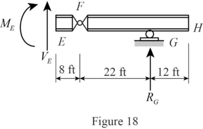
Find the equation of moment at E of portion AE.

$\begin{array}{l}{R}_G\left(30\right)+M_E=0\\ M_E=0\end{array}$

Consider portion EF $\left(72<x\le 80\text{ft}\right)$

Find the equation of moment at E for portion EF.

Apply a 1 kip in the portion DF from A.

Sketch the free body diagram of the section AC as shown in Figure 19.

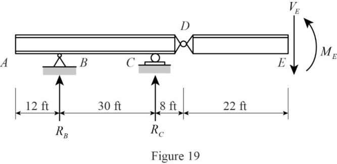
Find the equation of moment at E of portion EF.

$\begin{array}{l}-R_B\left(60\right)-R_C\left(30\right)+M_E=0\\ M_E=\left(0.0121x-0.877\right)\left(60\right)+\left(4.15-0.0576x\right)\left(30\right)\\ M_E=0.726x-52.62+124.5-1.728x\\ M_E=72-x\end{array}$

Consider portion FH $\left(80\le x\le 114\text{ft}\right)$

Find the equation of moment at E for portion FH.

Apply a 1 kip in the portion FH from A.

Sketch the free body diagram of the section AC as shown in Figure 20.

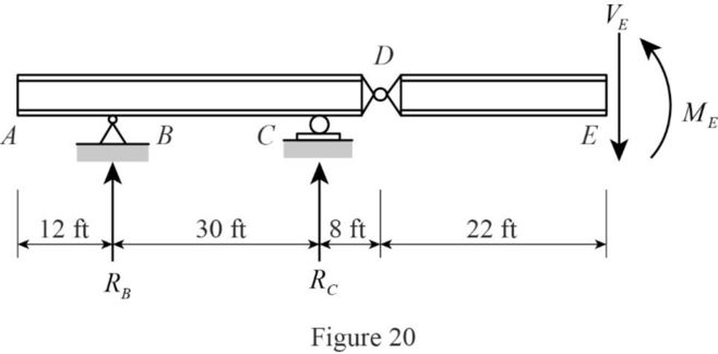
Find the equation of moment at D of portion FH.

$\begin{array}{l}-R_B\left(60\right)-R_C\left(30\right)+M_E=0\\ M_E=\left(0.4534-0.0045x\right)\left(60\right)+\left(0.021x-2.14\right)\left(30\right)\\ M_E=27.204-0.27x+0.63x-64.2\\ M_E=0.36x-37\end{array}$

Thus, the equations of the influence line for $M_C$ are,

$M_E=00\le x\le 72\text{ft}$        (16)

$M_C=72-x72\text{ft}\le x\le 80\text{ft}$        (17)

$M_E=0.36x-3780\text{ft}\le x\le 114\text{ft}$        (18)

Find the value of influence line ordinate of $R_C$ for various points of x using the Equations (16), (17), and (18) and summarize the value as in Table 6.

Points	x $\left(\text{ft}\right)$	$M_E$
A	0	0
$B$	12	0
C	42	0
D	50	0
E	72	0
F	80	‑8
G	102	0
H	114	4.04

Draw the influence lines for $M_E$ using Table 5 as shown in Figure 21.

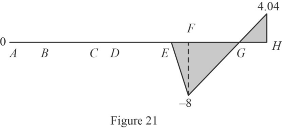
Refer Figure 21.

Determine the moment at E.

$\begin{array}{c}{M}_E=w\left[\frac{1}{2}\left(-8\right)\left(102-72\right)+\frac{1}{2}\left(4.04\right)\left(114-102\right)\right]\\ =2\left(-120+24.24\right)\\ =191.52\text{ft-k}\end{array}$

Therefore, the moment at E is $\underset{\_}{191.52\text{ft-k}}$.