Statistics for Business and Economics (13th Edition)
13th Edition
ISBN: 9780134506593
Author: James T. McClave, P. George Benson, Terry Sincich
Publisher: PEARSON
expand_more
expand_more
format_list_bulleted
Concept explainers
Videos
Textbook Question
Chapter 11.2, Problem 11.15LM
Refer to Exercise 11.14. After the least squares line has been obtained, the table below (which is similar to Table 11.2 can be used for (1) comparing the observed and the predicted values of y and (2) computing SSE
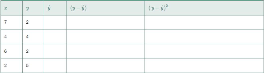

a. Complete the table.
b. Plot the least squares line on a
c. Show that SSE is larger for the line in part b than it is for the least squares line.
Expert Solution & Answer
Want to see the full answer?
Check out a sample textbook solution
Students have asked these similar questions
The average miles per gallon for a sample of 40 cars of model SX last year was 32.1, with a population standard deviation of 3.8. A sample of 40 cars from this year’s model SX has an average of 35.2 mpg, with a population standard deviation of 5.4.
Find a 99 percent confidence interval for the difference in average mpg for this car brand (this year’s model minus last year’s).Find a 99 percent confidence interval for the difference in average mpg for last year’s model minus this year’s. What does the negative difference mean?
A special interest group reports a tiny margin of error (plus or minus 0.04 percent) for its online survey based on 50,000 responses. Is the margin of error legitimate? (Assume that the group’s math is correct.)
Suppose that 73 percent of a sample of 1,000 U.S. college students drive a used car as opposed to a new car or no car at all.
Find an 80 percent confidence interval for the percentage of all U.S. college students who drive a used car.What sample size would cut this margin of error in half?
Chapter 11 Solutions
Statistics for Business and Economics (13th Edition)
Ch. 11.1 - In each case, graph the line that passes through...Ch. 11.1 - Give the slope and y-intercept for each of the...Ch. 11.1 - The equation for a straight line (deterministic...Ch. 11.1 - Refer to Exercise 11.3. Find the equations of the...Ch. 11.1 - Plot the following lines: a. y 4 + x b. y = 5 2x...Ch. 11.1 - Give the slope and y-intercept for each of the...Ch. 11.1 - Prob. 11.7LMCh. 11.1 - Prob. 11.8LMCh. 11.1 - If a straight-line probabilistic relationship...Ch. 11.1 - Congress voting on women's issues. The American...
Ch. 11.1 - Best-paid CEOs. Refer to Glassdoor Economic...Ch. 11.1 - Estimating repair and replacement costs of water...Ch. 11.1 - Forecasting movie revenues with Twitter. A study...Ch. 11.2 - The following table is similar to Table 11.2.It is...Ch. 11.2 - Refer to Exercise 11.14. After the least squares...Ch. 11.2 - Construct a scatterplot for the data in the...Ch. 11.2 - Consider the following pairs of measurements: a....Ch. 11.2 - Use the applet Regression by Eye to explore the...Ch. 11.2 - In business, do nice guys finish first or last?...Ch. 11.2 - State Math SAT scores. Refer to the data on...Ch. 11.2 - Lobster fishing study. Refer to the Bulletin of...Ch. 11.2 - Repair and replacement costs of water pipes. Refer...Ch. 11.2 - Joint Strike Fighter program. The Joint Strike...Ch. 11.2 - Software millionaires and birthdays. In Outliers:...Ch. 11.2 - Prob. 11.24ACICh. 11.2 - Ranking driving performance of professional...Ch. 11.2 - Sweetness of orange juice. The quality of the...Ch. 11.2 - Forecasting movie revenues with Twitter. Marketers...Ch. 11.2 - Charisma of top-level leaders. According to a...Ch. 11.2 - Ran kings of research universities. Refer to the...Ch. 11.2 - Prob. 11.30ACACh. 11.3 - Visually compare the scatterplots shown below. If...Ch. 11.3 - Calculate SSE and s2 for each of the following...Ch. 11.3 - Suppose you fit a least squares line to 26 data...Ch. 11.3 - Refer to Exercise 11.14 (p. 629). Calculate SSE,...Ch. 11.3 - Do nice guys really finish last in business? Refer...Ch. 11.3 - State Math SAT scores. Refer to the simple linear...Ch. 11.3 - Prob. 11.37ACBCh. 11.3 - Prob. 11.38ACBCh. 11.3 - Prob. 11.39ACBCh. 11.3 - Prob. 11.40ACICh. 11.3 - Prob. 11.41ACICh. 11.3 - Sweetness of orange juice. Refer to the study of...Ch. 11.3 - Rankings of research universities. Refer to the...Ch. 11.3 - Life tests of cutting tools. To Improve the...Ch. 11.4 - Construct both a 95% and a 90% confidence interval...Ch. 11.4 - Consider the following pairs of observations: a....Ch. 11.4 - Refer to Exercise 11.46. Construct an 80% and a...Ch. 11.4 - Do the accompanying data provide sufficient...Ch. 11.4 - State Math SAT Scores. Refer to the SPSS simple...Ch. 11.4 - Lobster fishing study. Refer to the Bulletin of...Ch. 11.4 - Prob. 11.51ACBCh. 11.4 - Prob. 11.52ACBCh. 11.4 - Estimating repair and replacement costs of water...Ch. 11.4 - Prob. 11.54ACBCh. 11.4 - Prob. 11.55ACICh. 11.4 - Beauty and electoral success. Are good looks an...Ch. 11.4 - Prob. 11.57ACICh. 11.4 - Prob. 11.58ACICh. 11.4 - Prob. 11.59ACICh. 11.4 - Prob. 11.60ACICh. 11.4 - Rankings of research universities. Refer to the...Ch. 11.4 - Prob. 11.62ACACh. 11.4 - Does elevation impact hitting performance in...Ch. 11.5 - Explain what each of the following sample...Ch. 11.5 - Describe the slope of the least squares line if a....Ch. 11.5 - Construct a scatterplot for each data set. Then...Ch. 11.5 - Calculate r2 for the least squares line in each of...Ch. 11.5 - Use the applet Correlation by Eye to explore the...Ch. 11.5 - In business, do nice guys finish first or last?...Ch. 11.5 - Going for it on fourth-down in the NFL Each week...Ch. 11.5 - Lobster fishing study. Refer to the Bulletin of...Ch. 11.5 - RateMyProfessors.com. A popular Web site among...Ch. 11.5 - Last name and acquisition timing. Refer to the...Ch. 11.5 - Women in top management. An empirical analysis of...Ch. 11.5 - Prob. 11.74ACICh. 11.5 - Prob. 11.75ACICh. 11.5 - Prob. 11.76ACICh. 11.5 - Prob. 11.77ACICh. 11.5 - Prob. 11.78ACICh. 11.5 - Evaluation of an imputation method for missing...Ch. 11.5 - Prob. 11.80ACICh. 11.5 - Prob. 11.81ACACh. 11.6 - Consider the followings of measurements: a...Ch. 11.6 - Consider the pairs of measurements shown in the...Ch. 11.6 - In fitting a least squares line to n = 10 data...Ch. 11.6 - Prob. 11.86ACBCh. 11.6 - Prob. 11.87ACBCh. 11.6 - Prob. 11.88ACBCh. 11.6 - Prob. 11.89ACBCh. 11.6 - Prob. 11.90ACBCh. 11.6 - Prob. 11.91ACICh. 11.6 - Ranking driving performance of professional...Ch. 11.6 - Spreading rate of spilled liquid Refer to the...Ch. 11.6 - Removing nitrogen from toxic wastewater. Highly...Ch. 11.6 - Predicting quit rates In manufacturing The reasons...Ch. 11.6 - Life tests of cutting tools Refer to the data...Ch. 11.7 - Prices of recycled materials. Prices of recycled...Ch. 11.7 - Thickness of dust on solar cells. The performance...Ch. 11.7 - Management research In Africa. The editors of the...Ch. 11.7 - An MBAs work-life balance. The importance of...Ch. 11 - In fitting a least squares line ton= 15 data...Ch. 11 - Consider the following sample data. a. Construct a...Ch. 11 - Consider the following 10 data points. a. Plot the...Ch. 11 - Drug controlled-release rate study. The effect of...Ch. 11 - Metaskills and career management. Effective...Ch. 11 - Burnout of human services professionals. Emotional...Ch. 11 - Retaliation against company whistle-blowers....Ch. 11 - Extending the life of an aluminum smelter pot. An...Ch. 11 - Diamonds sold at retail. Refer to the Journal of...Ch. 11 - Sports news on local TV broadcasts. The Sports...Ch. 11 - Evaluating managerial success. An observational...Ch. 11 - Doctors and ethics. Refer to the Journal of...Ch. 11 - FCAT scores and poverty. In the state of Florida,...Ch. 11 - Monetary values of NFL teams. Refer to the Forbes...Ch. 11 - Evaluating a truck weigh-in-motion program. The...Ch. 11 - Energy efficiency of buildings. Firms conscious of...Ch. 11 - Forecasting managerial needs. Managers are an...Ch. 11 - Prob. 11.118ACACh. 11 - Prob. 11.119CTCCh. 11 - Prob. 11.120CTC
Knowledge Booster


Learn more about
Need a deep-dive on the concept behind this application? Look no further. Learn more about this topic, statistics and related others by exploring similar questions and additional content below.Similar questions
- You want to compare the average number of tines on the antlers of male deer in two nearby metro parks. A sample of 30 deer from the first park shows an average of 5 tines with a population standard deviation of 3. A sample of 35 deer from the second park shows an average of 6 tines with a population standard deviation of 3.2. Find a 95 percent confidence interval for the difference in average number of tines for all male deer in the two metro parks (second park minus first park).Do the parks’ deer populations differ in average size of deer antlers?arrow_forwardSuppose that you want to increase the confidence level of a particular confidence interval from 80 percent to 95 percent without changing the width of the confidence interval. Can you do it?arrow_forwardA random sample of 1,117 U.S. college students finds that 729 go home at least once each term. Find a 98 percent confidence interval for the proportion of all U.S. college students who go home at least once each term.arrow_forward
- Suppose that you make two confidence intervals with the same data set — one with a 95 percent confidence level and the other with a 99.7 percent confidence level. Which interval is wider?Is a wide confidence interval a good thing?arrow_forwardIs it true that a 95 percent confidence interval means you’re 95 percent confident that the sample statistic is in the interval?arrow_forwardTines can range from 2 to upwards of 50 or more on a male deer. You want to estimate the average number of tines on the antlers of male deer in a nearby metro park. A sample of 30 deer has an average of 5 tines, with a population standard deviation of 3. Find a 95 percent confidence interval for the average number of tines for all male deer in this metro park.Find a 98 percent confidence interval for the average number of tines for all male deer in this metro park.arrow_forward
- Based on a sample of 100 participants, the average weight loss the first month under a new (competing) weight-loss plan is 11.4 pounds with a population standard deviation of 5.1 pounds. The average weight loss for the first month for 100 people on the old (standard) weight-loss plan is 12.8 pounds, with population standard deviation of 4.8 pounds. Find a 90 percent confidence interval for the difference in weight loss for the two plans( old minus new) Whats the margin of error for your calculated confidence interval?arrow_forwardA 95 percent confidence interval for the average miles per gallon for all cars of a certain type is 32.1, plus or minus 1.8. The interval is based on a sample of 40 randomly selected cars. What units represent the margin of error?Suppose that you want to decrease the margin of error, but you want to keep 95 percent confidence. What should you do?arrow_forward3. (i) Below is the R code for performing a X2 test on a 2×3 matrix of categorical variables called TestMatrix: chisq.test(Test Matrix) (a) Assuming we have a significant result for this procedure, provide the R code (including any required packages) for an appropriate post hoc test. (b) If we were to apply this technique to a 2 × 2 case, how would we adapt the code in order to perform the correct test? (ii) What procedure can we use if we want to test for association when we have ordinal variables? What code do we use in R to do this? What package does this command belong to? (iii) The following code contains the initial steps for a scenario where we are looking to investigate the relationship between age and whether someone owns a car by using frequencies. There are two issues with the code - please state these. Row3<-c(75,15) Row4<-c(50,-10) MortgageMatrix<-matrix(c(Row1, Row4), byrow=T, nrow=2, MortgageMatrix dimnames=list(c("Yes", "No"), c("40 or older","<40")))…arrow_forward
- Describe the situation in which Fisher’s exact test would be used?(ii) When do we use Yates’ continuity correction (with respect to contingencytables)?[2 Marks] 2. Investigate, checking the relevant assumptions, whether there is an associationbetween age group and home ownership based on the sample dataset for atown below:Home Owner: Yes NoUnder 40 39 12140 and over 181 59Calculate and evaluate the effect size.arrow_forwardNot use ai pleasearrow_forwardNeed help with the following statistic problems.arrow_forward
arrow_back_ios
SEE MORE QUESTIONS
arrow_forward_ios
Recommended textbooks for you
 Linear Algebra: A Modern IntroductionAlgebraISBN:9781285463247Author:David PoolePublisher:Cengage Learning
 Elementary Linear Algebra (MindTap Course List)AlgebraISBN:9781305658004Author:Ron LarsonPublisher:Cengage Learning
 Glencoe Algebra 1, Student Edition, 9780079039897...AlgebraISBN:9780079039897Author:CarterPublisher:McGraw Hill
 Big Ideas Math A Bridge To Success Algebra 1: Stu...AlgebraISBN:9781680331141Author:HOUGHTON MIFFLIN HARCOURTPublisher:Houghton Mifflin Harcourt
 Holt Mcdougal Larson Pre-algebra: Student Edition...AlgebraISBN:9780547587776Author:HOLT MCDOUGALPublisher:HOLT MCDOUGAL
 Functions and Change: A Modeling Approach to Coll...AlgebraISBN:9781337111348Author:Bruce Crauder, Benny Evans, Alan NoellPublisher:Cengage Learning
Linear Algebra: A Modern Introduction
Algebra
ISBN:9781285463247
Author:David Poole
Publisher:Cengage Learning
Elementary Linear Algebra (MindTap Course List)
Algebra
ISBN:9781305658004
Author:Ron Larson
Publisher:Cengage Learning
Glencoe Algebra 1, Student Edition, 9780079039897...
Algebra
ISBN:9780079039897
Author:Carter
Publisher:McGraw Hill
Big Ideas Math A Bridge To Success Algebra 1: Stu...
Algebra
ISBN:9781680331141
Author:HOUGHTON MIFFLIN HARCOURT
Publisher:Houghton Mifflin Harcourt
Holt Mcdougal Larson Pre-algebra: Student Edition...
Algebra
ISBN:9780547587776
Author:HOLT MCDOUGAL
Publisher:HOLT MCDOUGAL
Functions and Change: A Modeling Approach to Coll...
Algebra
ISBN:9781337111348
Author:Bruce Crauder, Benny Evans, Alan Noell
Publisher:Cengage Learning
Correlation Vs Regression: Difference Between them with definition & Comparison Chart; Author: Key Differences;https://www.youtube.com/watch?v=Ou2QGSJVd0U;License: Standard YouTube License, CC-BY
Correlation and Regression: Concepts with Illustrative examples; Author: LEARN & APPLY : Lean and Six Sigma;https://www.youtube.com/watch?v=xTpHD5WLuoA;License: Standard YouTube License, CC-BY