
Concept explainers
a)
To determine: The fraction defective in each sample.
Introduction: Quality is a measure of excellence or a state of being free from deficiencies, defects and important variations. It is obtained by consistent and strict commitment to certain standards to attain uniformity of a product to satisfy consumers’ requirement.
a)
Answer to Problem 5P
Explanation of Solution
Given information:
| Sample | 1 | 2 | 3 | 4 |
| Number with errors | 4 | 2 | 5 | 9 |
Calculation of fraction defective in each sample:
| n | 200 | |||
| Sample | 1 | 2 | 3 | 4 |
| Number with errors | 4 | 2 | 5 | 9 |
| Prop defective | 0.02 | 0.01 | 0.025 | 0.045 |
Excel Worksheet:
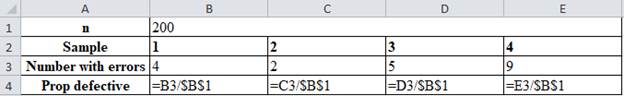
The proportion defective is calculated by dividing the number of errors with the number of samples. For sample 1, the number of errors 4 is divided by 200 which give 0.02 as prop defective.
Hence, the fraction defective is shown in Table 1.
b)
To determine: The estimation for fraction defective when true fraction defective for the process is unknown.
Introduction: Quality is a measure of excellence or a state of being free from deficiencies, defects and important variations. It is obtained by consistent and strict commitment to certain standards to attain uniformity of a product to satisfy consumers’ requirement.
b)
Answer to Problem 5P
Explanation of Solution
Given information:
| Sample | 1 | 2 | 3 | 4 |
| Number with errors | 4 | 2 | 5 | 9 |
Calculation of fraction defective:
The fraction defective is calculated when true fraction defective is unknown.
Total number of defective is calculated by adding the number of errors, (4+2+5+9) which accounts to 20
The fraction defective is calculated by dividing total number of defective with total number of observation which is 20 is divided with the product of 4 and 200 which is 0.025.
Hence, the fraction defective is 0.025.
c)
To determine: The estimate of mean and standard deviation of the sampling distribution of fraction defective for samples for the size.
Introduction:
Control chart:
It is a graph used to analyze the process change over a time period. A control chart has a upper control limit, and lower control which are used plot the time order.
c)
Answer to Problem 5P
Explanation of Solution
Given information:
| Sample | 1 | 2 | 3 | 4 |
| Number with errors | 4 | 2 | 5 | 9 |
Estimate of mean and standard deviation of the sampling distribution:
Mean = 0.025 (from equation (1))
The estimate for mean is shown in equation (1) and standard deviation is calculated by substituting the value which yields 0.011.
Hence, estimate of mean and standard deviation of the sampling distribution is 0.025 and 0.011.
d)
To determine: The control limits that would give an alpha risk of 0.03 for the process.
Introduction:
Control chart:
It is a graph used to analyze the process change over a time period. A control chart has a upper control limit, and lower control which are used plot the time order.
d)
Answer to Problem 5P
Explanation of Solution
Given information:
| Sample | 1 | 2 | 3 | 4 |
| Number with errors | 4 | 2 | 5 | 9 |
Control limits that would give an alpha risk of 0.03 for the process:
0.015 is in each tail and using z-factor table, value that corresponds to 0.5000 – 0.0150 is 0.4850 which is z = 2.17.
The UCL is calculated by adding 0.025 with the product of 2.17 and 0.011 which gives 0.0489 and LCL is calculated by subtracting 0.025 with the product of 2.17 and 0.011 which yields 0.0011.
Hence, the control limits that would give an alpha risk of 0.03 for the process are 0.0489 and 0.0011.
e)
To determine: The alpha risks that control limits 0.47 and 0.003 will provide.
Introduction:
Control chart:
It is a graph used to analyze the process change over a time period. A control chart has a upper control limit, and lower control which are used plot the time order.
e)
Answer to Problem 5P
Explanation of Solution
Given information:
| Sample | 1 | 2 | 3 | 4 |
| Number with errors | 4 | 2 | 5 | 9 |
Alpha risks that control limits 0.47 and 0.003 will provide:
The following equation z value can be calculated,
From z factor table, the probability value which corresponds to z = 2.00 is 0.4772, on each tail,
0.0228 is observed on each tail and doubling the value gives 0.0456 which is the alpha risk.
Hence, alpha risks that control limits 0.47 and 0.003 will provide is 0.0456
f)
To determine: Whether the process is in control when using 0.047 and 0.003.
Introduction:
Control chart:
It is a graph used to analyze the process change over a time period. A control chart has an upper control limit, and lower control which are used plot the time order.
f)
Answer to Problem 5P
Explanation of Solution
Given information:
| Sample | 1 | 2 | 3 | 4 |
| Number with errors | 4 | 2 | 5 | 9 |
Calculation of fraction defective in each sample:
| n | 200 | |||
| Sample | 1 | 2 | 3 | 4 |
| Number with errors | 4 | 2 | 5 | 9 |
| Prop defective | 0.02 | 0.01 | 0.025 | 0.045 |
UCL = 0.047 & LCL = 0.003
Graph:
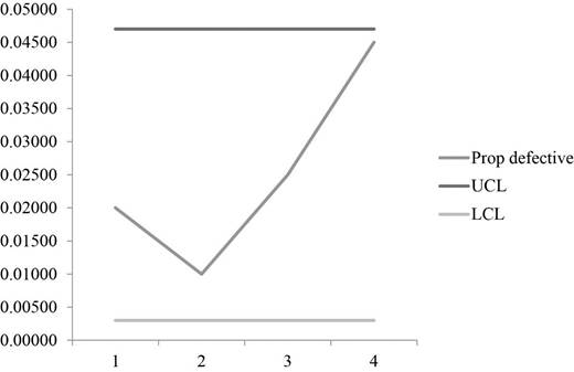
A graph is plotted using UCL, LCL and prop defective values which show that all the sample points are well within the control limits which makes the process to be in control.
Hence, the process is within control for the limits 0.047 & 0.003.
g)
To determine: The mean and standard deviation of the sampling distribution.
Introduction:
Control chart:
It is a graph used to analyze the process change over a time period. A control chart has a upper control limit, and lower control which are used plot the time order.
g)
Answer to Problem 5P
Explanation of Solution
Given information:
| Sample | 1 | 2 | 3 | 4 |
| Number with errors | 4 | 2 | 5 | 9 |
Long run fraction defective of the process is 0.02
Calculation of mean and standard deviation of the sampling distribution:
Fraction defective in each sample:
| n | 200 | |||
| Sample | 1 | 2 | 3 | 4 |
| Number with errors | 4 | 2 | 5 | 9 |
| Prop defective | 0.02 | 0.01 | 0.025 | 0.045 |
The mean is calculated by taking average for the proportion defective,
The values of the proportion defective are added and divided by 4 which give 0.02.
The standard deviation is calculated using the formula,
The standard deviation is calculated by substituting the values in the above formula and taking square root for the resultant value which yields 0.099.
Hence, mean and standard deviation of the sampling distribution is 0.02&0.0099.
h)
To construct: A control chart using two sigma control limits and check whether the process is in control.
Introduction:
Control chart:
It is a graph used to analyze the process change over a time period. A control chart has a upper control limit, and lower control which are used plot the time order.
h)
Answer to Problem 5P
Explanation of Solution
Given information:
| Sample | 1 | 2 | 3 | 4 |
| Number with errors | 4 | 2 | 5 | 9 |
Fraction defective in each sample:
| n | 200 | |||
| Sample | 1 | 2 | 3 | 4 |
| Number with errors | 4 | 2 | 5 | 9 |
| Prop defective | 0.02 | 0.01 | 0.025 | 0.045 |
Calculation of control limits:
The control limits are calculated using the above formula and substituting the values and taking square root gives the control limits of the UCL and LCL which are 0.0398 and 0.0002 respectively.
Graph:
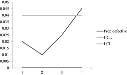
A graph is plotted using the fraction defective, UCL and LCL values which shows that one sample points is beyond the control region which makes the process to be out of control.
Hence, control chart is constructed using two-sigma control limits and the chart shows that the process is not in control.
Want to see more full solutions like this?
Chapter 10 Solutions
OPERATIONS MANAGEMENT(LL)-W/CONNECT


- northeastern insurance company is considering opening an office in the US. The two cities under consideration are going to be Philadelphia New York. Factor ratings (higher scores are better) are in the table. The best location for northeastern insurance company to open would be which with a total weighted score of ? (response rounded to two decimal places)arrow_forwardWhen football fans watch a game, they believe the other side commits more infractions on the field than does their own team. This favoritism can best be termed _____. Group of answer choices A. ethnocentrism B. the fundamental attribution error C. the affiliation bias D. marginalizationarrow_forwardWhen football fans watch a game, they believe the other side commits more infractions on the field than does their own team. This favoritism can best be termed _____. Group of answer choices ethnocentrism the fundamental attribution error the affiliation bias marginalizationarrow_forward
- Which of the following best describes the differences between egalitarianism and hierarchy as cultural values in negotiation? Group of answer choices A. Egalitarian cultures communicate directly; hierarchical cultures communicate indirectly. B. Egalitarian cultures treat people equally; hierarchical cultures discriminate among people. C. Egalitarian cultures divide things equally; hierarchical cultures divide things according to merit and status. D. Egalitarian cultures believe that status is permeable through effort and achievement; hierarchical cultures believe that superiors should take care of the needs of subordinates.arrow_forwardWhich of the following best describes the differences between individualism and collectivism as cultural values in negotiation? Group of answer choices A. Individualists see themselves as autonomous entities; collectivists see themselves in relation to others. B. Individualists prefer to work in groups; collectivists prefer to work alone. C. Individualists are cooperative; collectivists are competitive. D. Individualists focus on relationships; collectivists focus on money.arrow_forwardWhen it comes to resolving conflict, managers from hierarchical cultures prefer _____. Group of answer choices A. to attribute a disagreeable person's behavior to an underlying disposition and desire formal dispute resolution procedures B. an interests model that relies on resolving underlying conflicts C. to regulate behavior via public shaming D. to defer to a higher status personarrow_forward
- The tripartite model of culture is based on three cultural prototypes that represent negotiators’ self-views and are highly correlated with particular geographic regions. Give an example of the three. Face Dignity Honorarrow_forwardThe personality and unique character of a social group is best known as its _____ and includes the values and norms shared by its members and encompasses the structure of its social, political, economic, and religious institutions. Group of answer choices group identity group potency group stereotype culturearrow_forwardagree or disagree with this post Face - “Face” or dignity in a negotiation has been called “one of an individual’s most sacred possessions.”102 Face is the value a person places on his or her public image, reputation, and status vis-à-vis other people in the negotiation. Direct threats to face in a negotiation include making ultimatums, criticisms, challenges, and insults (Thompson, 2019). A good example of face is when I go to the negotiation table with a counterpart that is known to be difficult or not as knowledgeable about the category as they should be, my approach wouldn't be to point out their weakness, I will respect their thought process, show consideration for their perspective, all while guiding the conversation in the direction of my intended negotiation strategy in hopes to achieve my desired outcome. Dignity - endorses views such as, “People should stand up for what they believe in, even when others disagree,” and “How much a person respects oneself is far more…arrow_forward
- 16:53 ◄ Mail 5G CSTUDY_Jan25_SCMH_O...Final_20250220143201.pdf CHOOSING FORECASTING MODELS gradienting are more mode. Yet when selecting a forecasting method, the door forecasts in fact, each of the three methods has different strength and can play important ing importance of the factors, such as the index and cast model, or a unified approach, ch del runs individual series separately A galable manufacturer is facing changes with demand fuctuations due to economiyapply make changes. Comment on why this has been the case and propose a forecasting approach that can be utilised t Question 13 ashit from a batch production process to a continuous flows to enhance efficiency. Critically analyse the trade- A public hospital in Free State is experiencing increasing patient wait times due to limited operacity. The hospital management is considering either expanding existing facilities orating more efficient Question 1.5 A farming consponsible for planting grain crops in Free State As expected…arrow_forwardHow can a college basketball coach use lean system strategies to improve the team's performance and win the national championship? What wastes can be eliminated from the team's training and equipment? How can performance data be used to adjust the team's strategy and tactics?arrow_forwardHow much does self-awareness influence the Interpersonal Trust Scale's results?arrow_forward
 Practical Management ScienceOperations ManagementISBN:9781337406659Author:WINSTON, Wayne L.Publisher:Cengage,