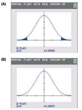
Babies’ Weights, Again Some sources report that the weights of full-term newborn babies have a mean of 7 pounds and a standard deviation of 0.6 pound and are Normally distributed. In the given outputs, the shaded areas (reported as p = ) represent the probability that the mean will be larger than 7.6 or smaller than 6.4. One of the outputs uses a sample size of 4, and one uses a sample size of 9. a. Which is which, and how do you know? b. These graphs are made so that they spread out to occupy the room on the face of the calculator. If they had the same horizontal axis, one would be taller and narrower than the other. Which one would that be, and why?
Babies’ Weights, Again Some sources report that the weights of full-term newborn babies have a mean of 7 pounds and a standard deviation of 0.6 pound and are Normally distributed. In the given outputs, the shaded areas (reported as p = ) represent the probability that the mean will be larger than 7.6 or smaller than 6.4. One of the outputs uses a sample size of 4, and one uses a sample size of 9. a. Which is which, and how do you know? b. These graphs are made so that they spread out to occupy the room on the face of the calculator. If they had the same horizontal axis, one would be taller and narrower than the other. Which one would that be, and why?
Solution Summary: The author identifies the outputs which display the probability for the sample size of 4 and 9.
Babies’ Weights, Again Some sources report that the weights of full-term newborn babies have a mean of 7 pounds and a standard deviation of 0.6 pound and are Normally distributed. In the given outputs, the shaded areas (reported as
p
=
) represent the probability that the mean will be larger than 7.6 or smaller than 6.4. One of the outputs uses a sample size of 4, and one uses a sample size of 9.
a. Which is which, and how do you know?
b. These graphs are made so that they spread out to occupy the room on the face of the calculator. If they had the same horizontal axis, one would be taller and narrower than the other. Which one would that be, and why?
Features Features Normal distribution is characterized by two parameters, mean (µ) and standard deviation (σ). When graphed, the mean represents the center of the bell curve and the graph is perfectly symmetric about the center. The mean, median, and mode are all equal for a normal distribution. The standard deviation measures the data's spread from the center. The higher the standard deviation, the more the data is spread out and the flatter the bell curve looks. Variance is another commonly used measure of the spread of the distribution and is equal to the square of the standard deviation.
08:34
◄ Classroom
07:59
Probs. 5-32/33
D
ا.
89
5-34. Determine the horizontal and vertical components
of reaction at the pin A and the normal force at the smooth
peg B on the member.
A
0,4 m
0.4 m
Prob. 5-34
F=600 N
fr
th
ar
0.
163586
5-37. The wooden plank resting between the buildings
deflects slightly when it supports the 50-kg boy. This
deflection causes a triangular distribution of load at its ends.
having maximum intensities of w, and wg. Determine w
and wg. each measured in N/m. when the boy is standing
3 m from one end as shown. Neglect the mass of the plank.
0.45 m
3 m
Examine the Variables: Carefully review and note the names of all variables in the dataset. Examples of these variables include:
Mileage (mpg)
Number of Cylinders (cyl)
Displacement (disp)
Horsepower (hp)
Research: Google to understand these variables.
Statistical Analysis: Select mpg variable, and perform the following statistical tests. Once you are done with these tests using mpg variable, repeat the same with hp
Mean
Median
First Quartile (Q1)
Second Quartile (Q2)
Third Quartile (Q3)
Fourth Quartile (Q4)
10th Percentile
70th Percentile
Skewness
Kurtosis
Document Your Results:
In RStudio: Before running each statistical test, provide a heading in the format shown at the bottom. “# Mean of mileage – Your name’s command”
In Microsoft Word: Once you've completed all tests, take a screenshot of your results in RStudio and paste it into a Microsoft Word document. Make sure that snapshots are very clear. You will need multiple snapshots. Also transfer these results to the…
Need a deep-dive on the concept behind this application? Look no further. Learn more about this topic, statistics and related others by exploring similar questions and additional content below.


 Glencoe Algebra 1, Student Edition, 9780079039897...AlgebraISBN:9780079039897Author:CarterPublisher:McGraw Hill