
Videos
(a)
Draw the time-series plot for the given data.
Identify the pattern.
(a)
Explanation of Solution
Step-by-step procedure to construct time-series plot is given below.
- Enter the data in columns A and B. Select the data.
- Click on Insert tab and then click on line.
- Select line with markers
The output is given below:
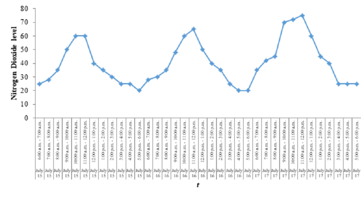
From the above time-series plot, it is clear that plot shows upward trend. Also, there exists seasonal pattern.
(b)
Find a multiple regression equation that represents seasonal effect using dummy variables for the given data.
(b)
Answer to Problem 25P
The regression equation is,
Explanation of Solution
Dummy variables are defined as given below:
Also, all the dummy variables are 0 when the reading time corresponds to 5:00 p.m. to 6:00 p.m.
The given data is entered as given below:
| Hourly Dummy Variables | |||||||||||||
| Date | Hour | yt | 1 | 2 | 3 | 4 | 5 | 6 | 7 | 8 | 9 | 10 | 11 |
| July 15 | 6:00 a.m. - 7:00 a.m. | 25 | 1 | 0 | 0 | 0 | 0 | 0 | 0 | 0 | 0 | 0 | 0 |
| July 15 | 7:00 a.m. - 8:00 a.m. | 28 | 0 | 1 | 0 | 0 | 0 | 0 | 0 | 0 | 0 | 0 | 0 |
| July 15 | 8:00 a.m. - 9:00 a.m. | 35 | 0 | 0 | 1 | 0 | 0 | 0 | 0 | 0 | 0 | 0 | 0 |
| July 15 | 9:00 a.m. - 10:00 a.m. | 50 | 0 | 0 | 0 | 1 | 0 | 0 | 0 | 0 | 0 | 0 | 0 |
| July 15 | 10:00 a.m. - 11:00 a.m. | 60 | 0 | 0 | 0 | 0 | 1 | 0 | 0 | 0 | 0 | 0 | 0 |
| July 15 | 11:00 a.m. - 12:00 p.m. | 60 | 0 | 0 | 0 | 0 | 0 | 1 | 0 | 0 | 0 | 0 | 0 |
| July 15 | 12:00 p.m. - 1:00 p.m. | 40 | 0 | 0 | 0 | 0 | 0 | 0 | 1 | 0 | 0 | 0 | 0 |
| July 15 | 1:00 p.m. - 2:00 p.m. | 35 | 0 | 0 | 0 | 0 | 0 | 0 | 0 | 1 | 0 | 0 | 0 |
| July 15 | 2:00 p.m. - 3:00 p.m. | 30 | 0 | 0 | 0 | 0 | 0 | 0 | 0 | 0 | 1 | 0 | 0 |
| July 15 | 3:00 p.m. - 4:00 p.m. | 25 | 0 | 0 | 0 | 0 | 0 | 0 | 0 | 0 | 0 | 1 | 0 |
| July 15 | 4:00 p.m. - 5:00 p.m. | 25 | 0 | 0 | 0 | 0 | 0 | 0 | 0 | 0 | 0 | 0 | 1 |
| July 15 | 5:00 p.m. - 6:00 p.m. | 20 | 0 | 0 | 0 | 0 | 0 | 0 | 0 | 0 | 0 | 0 | 0 |
| July 16 | 6:00 a.m. - 7:00 a.m. | 28 | 1 | 0 | 0 | 0 | 0 | 0 | 0 | 0 | 0 | 0 | 0 |
| July 16 | 7:00 a.m. - 8:00 a.m. | 30 | 0 | 1 | 0 | 0 | 0 | 0 | 0 | 0 | 0 | 0 | 0 |
| July 16 | 8:00 a.m. - 9:00 a.m. | 35 | 0 | 0 | 1 | 0 | 0 | 0 | 0 | 0 | 0 | 0 | 0 |
| July 16 | 9:00 a.m. - 10:00 a.m. | 48 | 0 | 0 | 0 | 1 | 0 | 0 | 0 | 0 | 0 | 0 | 0 |
| July 16 | 10:00 a.m. - 11:00 a.m. | 60 | 0 | 0 | 0 | 0 | 1 | 0 | 0 | 0 | 0 | 0 | 0 |
| July 16 | 11:00 a.m. - 12:00 p.m. | 65 | 0 | 0 | 0 | 0 | 0 | 1 | 0 | 0 | 0 | 0 | 0 |
| July 16 | 12:00 p.m. - 1:00 p.m. | 50 | 0 | 0 | 0 | 0 | 0 | 0 | 1 | 0 | 0 | 0 | 0 |
| July 16 | 1:00 p.m. - 2:00 p.m. | 40 | 0 | 0 | 0 | 0 | 0 | 0 | 0 | 1 | 0 | 0 | 0 |
| July 16 | 2:00 p.m. - 3:00 p.m. | 35 | 0 | 0 | 0 | 0 | 0 | 0 | 0 | 0 | 1 | 0 | 0 |
| July 16 | 3:00 p.m. - 4:00 p.m. | 25 | 0 | 0 | 0 | 0 | 0 | 0 | 0 | 0 | 0 | 1 | 0 |
| July 16 | 4:00 p.m. - 5:00 p.m. | 20 | 0 | 0 | 0 | 0 | 0 | 0 | 0 | 0 | 0 | 0 | 1 |
| July 16 | 5:00 p.m. - 6:00 p.m. | 20 | 0 | 0 | 0 | 0 | 0 | 0 | 0 | 0 | 0 | 0 | 0 |
| July 17 | 6:00 a.m. - 7:00 a.m. | 35 | 1 | 0 | 0 | 0 | 0 | 0 | 0 | 0 | 0 | 0 | 0 |
| July 17 | 7:00 a.m. - 8:00 a.m. | 42 | 0 | 1 | 0 | 0 | 0 | 0 | 0 | 0 | 0 | 0 | 0 |
| July 17 | 8:00 a.m. - 9:00 a.m. | 45 | 0 | 0 | 1 | 0 | 0 | 0 | 0 | 0 | 0 | 0 | 0 |
| July 17 | 9:00 a.m. - 10:00 a.m. | 70 | 0 | 0 | 0 | 1 | 0 | 0 | 0 | 0 | 0 | 0 | 0 |
| July 17 | 10:00 a.m. - 11:00 a.m. | 72 | 0 | 0 | 0 | 0 | 1 | 0 | 0 | 0 | 0 | 0 | 0 |
| July 17 | 11:00 a.m. - 12:00 p.m. | 75 | 0 | 0 | 0 | 0 | 0 | 1 | 0 | 0 | 0 | 0 | 0 |
| July 17 | 12:00 p.m. - 1:00 p.m. | 60 | 0 | 0 | 0 | 0 | 0 | 0 | 1 | 0 | 0 | 0 | 0 |
| July 17 | 1:00 p.m. - 2:00 p.m. | 45 | 0 | 0 | 0 | 0 | 0 | 0 | 0 | 1 | 0 | 0 | 0 |
| July 17 | 2:00 p.m. - 3:00 p.m. | 40 | 0 | 0 | 0 | 0 | 0 | 0 | 0 | 0 | 1 | 0 | 0 |
| July 17 | 3:00 p.m. - 4:00 p.m. | 25 | 0 | 0 | 0 | 0 | 0 | 0 | 0 | 0 | 0 | 1 | 0 |
| July 17 | 4:00 p.m. - 5:00 p.m. | 25 | 0 | 0 | 0 | 0 | 0 | 0 | 0 | 0 | 0 | 0 | 1 |
| July 17 | 5:00 p.m. - 6:00 p.m. | 25 | 0 | 0 | 0 | 0 | 0 | 0 | 0 | 0 | 0 | 0 | 0 |
Step-by-step procedure to obtain multiple linear regression line is given below.
- Enter the data in columns A to M.
- Click on Data tab and then Data Analysis.
- Select Regression and click ok.
- In Input Y
Range select, $B$2:$B$37 and Input X Range select $C$2:$M$37 - Click Ok.
The output is given below:
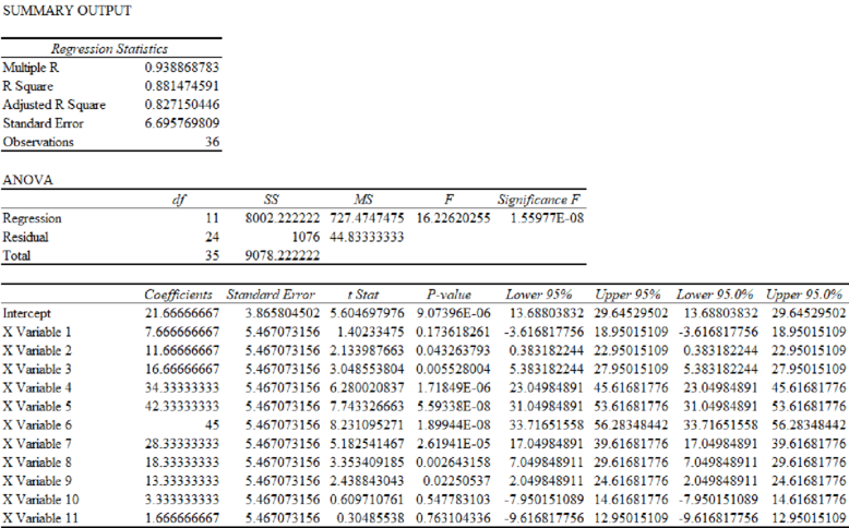
From the output the regression equation is,
Here, X Variable 1 represents Hour1, X Variable 2 represents Hour2, … X variable 11 represents Hour11.
(c)
Find the estimates of the levels of nitrogen for July 18 using the model developed in part (b).
(c)
Explanation of Solution
From part (b), the regression equation is,
Forecast for July 18 is obtained as given below:
| Hourly forecast | Calculation | |
| Hour1 | 29.34 | |
| Hour2 | 33.34 | |
| Hour3 | 38.34 | |
| Hour4 | 56 | |
| Hour5 | 64 | |
| Hour6 | 66.67 | |
| Hour7 | 50 | |
| Hour8 | 40 | |
| Hour9 | 35 | |
| Hour10 | 25 | |
| Hour11 | 23.34 | |
| Hour12 | 21.67 | 21.67 |
(d)
Construct a multiple regression equation that represents seasonal effect using dummy variables and a t variable for the given data.
(d)
Answer to Problem 25P
The regression equation is,
Explanation of Solution
Create a variable t such that t = 1 for hour 1 on July 15, t = 2 for hour 2 on July 2, …, t = 36 for hour 12 on July 18.
The given data is entered as given below:
| Hourly Dummy Variables | ||||||||||||||
| Date | Hour | yt | 1 | 2 | 3 | 4 | 5 | 6 | 7 | 8 | 9 | 10 | 11 | t |
| July 15 | 6:00 a.m. - 7:00 a.m. | 25 | 1 | 0 | 0 | 0 | 0 | 0 | 0 | 0 | 0 | 0 | 0 | 1 |
| July 15 | 7:00 a.m. - 8:00 a.m. | 28 | 0 | 1 | 0 | 0 | 0 | 0 | 0 | 0 | 0 | 0 | 0 | 2 |
| July 15 | 8:00 a.m. - 9:00 a.m. | 35 | 0 | 0 | 1 | 0 | 0 | 0 | 0 | 0 | 0 | 0 | 0 | 3 |
| July 15 | 9:00 a.m. - 10:00 a.m. | 50 | 0 | 0 | 0 | 1 | 0 | 0 | 0 | 0 | 0 | 0 | 0 | 4 |
| July 15 | 10:00 a.m. - 11:00 a.m. | 60 | 0 | 0 | 0 | 0 | 1 | 0 | 0 | 0 | 0 | 0 | 0 | 5 |
| July 15 | 11:00 a.m. - 12:00 p.m. | 60 | 0 | 0 | 0 | 0 | 0 | 1 | 0 | 0 | 0 | 0 | 0 | 6 |
| July 15 | 12:00 p.m. - 1:00 p.m. | 40 | 0 | 0 | 0 | 0 | 0 | 0 | 1 | 0 | 0 | 0 | 0 | 7 |
| July 15 | 1:00 p.m. - 2:00 p.m. | 35 | 0 | 0 | 0 | 0 | 0 | 0 | 0 | 1 | 0 | 0 | 0 | 8 |
| July 15 | 2:00 p.m. - 3:00 p.m. | 30 | 0 | 0 | 0 | 0 | 0 | 0 | 0 | 0 | 1 | 0 | 0 | 9 |
| July 15 | 3:00 p.m. - 4:00 p.m. | 25 | 0 | 0 | 0 | 0 | 0 | 0 | 0 | 0 | 0 | 1 | 0 | 10 |
| July 15 | 4:00 p.m. - 5:00 p.m. | 25 | 0 | 0 | 0 | 0 | 0 | 0 | 0 | 0 | 0 | 0 | 1 | 11 |
| July 15 | 5:00 p.m. - 6:00 p.m. | 20 | 0 | 0 | 0 | 0 | 0 | 0 | 0 | 0 | 0 | 0 | 0 | 12 |
| July 16 | 6:00 a.m. - 7:00 a.m. | 28 | 1 | 0 | 0 | 0 | 0 | 0 | 0 | 0 | 0 | 0 | 0 | 13 |
| July 16 | 7:00 a.m. - 8:00 a.m. | 30 | 0 | 1 | 0 | 0 | 0 | 0 | 0 | 0 | 0 | 0 | 0 | 14 |
| July 16 | 8:00 a.m. - 9:00 a.m. | 35 | 0 | 0 | 1 | 0 | 0 | 0 | 0 | 0 | 0 | 0 | 0 | 15 |
| July 16 | 9:00 a.m. - 10:00 a.m. | 48 | 0 | 0 | 0 | 1 | 0 | 0 | 0 | 0 | 0 | 0 | 0 | 16 |
| July 16 | 10:00 a.m. - 11:00 a.m. | 60 | 0 | 0 | 0 | 0 | 1 | 0 | 0 | 0 | 0 | 0 | 0 | 17 |
| July 16 | 11:00 a.m. - 12:00 p.m. | 65 | 0 | 0 | 0 | 0 | 0 | 1 | 0 | 0 | 0 | 0 | 0 | 18 |
| July 16 | 12:00 p.m. - 1:00 p.m. | 50 | 0 | 0 | 0 | 0 | 0 | 0 | 1 | 0 | 0 | 0 | 0 | 19 |
| July 16 | 1:00 p.m. - 2:00 p.m. | 40 | 0 | 0 | 0 | 0 | 0 | 0 | 0 | 1 | 0 | 0 | 0 | 20 |
| July 16 | 2:00 p.m. - 3:00 p.m. | 35 | 0 | 0 | 0 | 0 | 0 | 0 | 0 | 0 | 1 | 0 | 0 | 21 |
| July 16 | 3:00 p.m. - 4:00 p.m. | 25 | 0 | 0 | 0 | 0 | 0 | 0 | 0 | 0 | 0 | 1 | 0 | 22 |
| July 16 | 4:00 p.m. - 5:00 p.m. | 20 | 0 | 0 | 0 | 0 | 0 | 0 | 0 | 0 | 0 | 0 | 1 | 23 |
| July 16 | 5:00 p.m. - 6:00 p.m. | 20 | 0 | 0 | 0 | 0 | 0 | 0 | 0 | 0 | 0 | 0 | 0 | 24 |
| July 17 | 6:00 a.m. - 7:00 a.m. | 35 | 1 | 0 | 0 | 0 | 0 | 0 | 0 | 0 | 0 | 0 | 0 | 25 |
| July 17 | 7:00 a.m. - 8:00 a.m. | 42 | 0 | 1 | 0 | 0 | 0 | 0 | 0 | 0 | 0 | 0 | 0 | 26 |
| July 17 | 8:00 a.m. - 9:00 a.m. | 45 | 0 | 0 | 1 | 0 | 0 | 0 | 0 | 0 | 0 | 0 | 0 | 27 |
| July 17 | 9:00 a.m. - 10:00 a.m. | 70 | 0 | 0 | 0 | 1 | 0 | 0 | 0 | 0 | 0 | 0 | 0 | 28 |
| July 17 | 10:00 a.m. - 11:00 a.m. | 72 | 0 | 0 | 0 | 0 | 1 | 0 | 0 | 0 | 0 | 0 | 0 | 29 |
| July 17 | 11:00 a.m. - 12:00 p.m. | 75 | 0 | 0 | 0 | 0 | 0 | 1 | 0 | 0 | 0 | 0 | 0 | 30 |
| July 17 | 12:00 p.m. - 1:00 p.m. | 60 | 0 | 0 | 0 | 0 | 0 | 0 | 1 | 0 | 0 | 0 | 0 | 31 |
| July 17 | 1:00 p.m. - 2:00 p.m. | 45 | 0 | 0 | 0 | 0 | 0 | 0 | 0 | 1 | 0 | 0 | 0 | 32 |
| July 17 | 2:00 p.m. - 3:00 p.m. | 40 | 0 | 0 | 0 | 0 | 0 | 0 | 0 | 0 | 1 | 0 | 0 | 33 |
| July 17 | 3:00 p.m. - 4:00 p.m. | 25 | 0 | 0 | 0 | 0 | 0 | 0 | 0 | 0 | 0 | 1 | 0 | 34 |
| July 17 | 4:00 p.m. - 5:00 p.m. | 25 | 0 | 0 | 0 | 0 | 0 | 0 | 0 | 0 | 0 | 0 | 1 | 35 |
| July 17 | 5:00 p.m. - 6:00 p.m. | 25 | 0 | 0 | 0 | 0 | 0 | 0 | 0 | 0 | 0 | 0 | 0 | 36 |
Step-by-step procedure to obtain multiple linear regression line is given below.
- Enter the data in columns A to N.
- Click on Data tab and then Data Analysis.
- Select Regression and click ok.
- In Input Y Range select, $B$2:$B$37 and Input X Range select $C$2:$N$37
- Click Ok.
The output is given below:
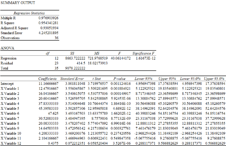
From the output the regression equation is,
Here, X Variable 1 represents Hour1, X Variable 2 represents Hour2,… X variable 11 represents Hour11 and X variable 12 represents t.
(e)
Calculate the estimates of the levels of nitrogen for July 18 using the model developed in part (d).
(e)
Explanation of Solution
From part (d), the regression equation is,
Forecast for July 18 is given below:
| Hourly forecast | T | Calculation | |
| 1 | 37 | 39.93 | |
| 2 | 38 | 43.93 | |
| 3 | 39 | 48.93 | |
| 4 | 40 | 66.6 | |
| 5 | 41 | 74.71 | |
| 6 | 42 | 77.28 | |
| 7 | 43 | 60.61 | |
| 8 | 44 | 50.61 | |
| 9 | 45 | 45.62 | |
| 10 | 46 | 35.62 | |
| 11 | 47 | 33.95 | |
| 12 | 48 | 32.29 |
(f)
Justify which of the models (b) or (d) is effective.
(f)
Answer to Problem 25P
Model (d) is preferred.
Explanation of Solution
For the multiple regression equation developed in part (b), MSE is obtained as given below:
| Date | Hour | yt | Forecast | Forecast Error | Squared Forecast Error |
| 15-Jul | 6:00 a.m. - 7:00 a.m. | 25 | 29.34 | -4.34 | 18.8356 |
| 15-Jul | 7:00 a.m. - 8:00 a.m. | 28 | 33.34 | -5.34 | 28.5156 |
| 15-Jul | 8:00 a.m. - 9:00 a.m. | 35 | 38.34 | -3.34 | 11.1556 |
| 15-Jul | 9:00 a.m. - 10:00 a.m. | 50 | 56 | -6 | 36 |
| 15-Jul | 10:00 a.m. - 11:00 a.m. | 60 | 64 | -4 | 16 |
| 15-Jul | 11:00 a.m. - 12:00 p.m. | 60 | 66.67 | -6.67 | 44.4889 |
| 15-Jul | 12:00 p.m. - 1:00 p.m. | 40 | 50 | -10 | 100 |
| 15-Jul | 1:00 p.m. - 2:00 p.m. | 35 | 40 | -5 | 25 |
| 15-Jul | 2:00 p.m. - 3:00 p.m. | 30 | 35 | -5 | 25 |
| 15-Jul | 3:00 p.m. - 4:00 p.m. | 25 | 25 | 0 | 0 |
| 15-Jul | 4:00 p.m. - 5:00 p.m. | 25 | 23.34 | 1.66 | 2.7556 |
| 15-Jul | 5:00 p.m. - 6:00 p.m. | 20 | 21.67 | -1.67 | 2.7889 |
| 16-Jul | 6:00 a.m. - 7:00 a.m. | 28 | 29.34 | -1.34 | 1.7956 |
| 16-Jul | 7:00 a.m. - 8:00 a.m. | 30 | 33.34 | -3.34 | 11.1556 |
| 16-Jul | 8:00 a.m. - 9:00 a.m. | 35 | 38.34 | -3.34 | 11.1556 |
| 16-Jul | 9:00 a.m. - 10:00 a.m. | 48 | 56 | -8 | 64 |
| 16-Jul | 10:00 a.m. - 11:00 a.m. | 60 | 64 | -4 | 16 |
| 16-Jul | 11:00 a.m. - 12:00 p.m. | 65 | 66.67 | -1.67 | 2.7889 |
| 16-Jul | 12:00 p.m. - 1:00 p.m. | 50 | 50 | 0 | 0 |
| 16-Jul | 1:00 p.m. - 2:00 p.m. | 40 | 40 | 0 | 0 |
| 16-Jul | 2:00 p.m. - 3:00 p.m. | 35 | 35 | 0 | 0 |
| 16-Jul | 3:00 p.m. - 4:00 p.m. | 25 | 25 | 0 | 0 |
| 16-Jul | 4:00 p.m. - 5:00 p.m. | 20 | 23.34 | -3.34 | 11.1556 |
| 16-Jul | 5:00 p.m. - 6:00 p.m. | 20 | 21.67 | -1.67 | 2.7889 |
| 17-Jul | 6:00 a.m. - 7:00 a.m. | 35 | 29.34 | 5.66 | 32.0356 |
| 17-Jul | 7:00 a.m. - 8:00 a.m. | 42 | 33.34 | 8.66 | 74.9956 |
| 17-Jul | 8:00 a.m. - 9:00 a.m. | 45 | 38.34 | 6.66 | 44.3556 |
| 17-Jul | 9:00 a.m. - 10:00 a.m. | 70 | 56 | 14 | 196 |
| 17-Jul | 10:00 a.m. - 11:00 a.m. | 72 | 64 | 8 | 64 |
| 17-Jul | 11:00 a.m. - 12:00 p.m. | 75 | 66.67 | 8.33 | 69.3889 |
| 17-Jul | 12:00 p.m. - 1:00 p.m. | 60 | 50 | 10 | 100 |
| 17-Jul | 1:00 p.m. - 2:00 p.m. | 45 | 40 | 5 | 25 |
| 17-Jul | 2:00 p.m. - 3:00 p.m. | 40 | 35 | 5 | 25 |
| 17-Jul | 3:00 p.m. - 4:00 p.m. | 25 | 25 | 0 | 0 |
| 17-Jul | 4:00 p.m. - 5:00 p.m. | 25 | 23.34 | 1.66 | 2.7556 |
| 17-Jul | 5:00 p.m. - 6:00 p.m. | 25 | 21.67 | 3.33 | 11.0889 |
| 1076.001 |
For the multiple regression equation developed in part (d), MSE is obtained as given below:
| Date | Hour | t | yt | Forecast | Forecast Error | Squared Forecast Error |
| 15-Jul | 6:00 a.m. - 7:00 a.m. | 1 | 25 | 24.09 | 0.91 | 0.8281 |
| 15-Jul | 7:00 a.m. - 8:00 a.m. | 2 | 28 | 28.09 | -0.09 | 0.0081 |
| 15-Jul | 8:00 a.m. - 9:00 a.m. | 3 | 35 | 33.09 | 1.91 | 3.6481 |
| 15-Jul | 9:00 a.m. - 10:00 a.m. | 4 | 50 | 50.76 | -0.76 | 0.5776 |
| 15-Jul | 10:00 a.m. - 11:00 a.m. | 5 | 60 | 58.87 | 1.13 | 1.2769 |
| 15-Jul | 11:00 a.m. - 12:00 p.m. | 6 | 60 | 61.44 | -1.44 | 2.0736 |
| 15-Jul | 12:00 p.m. - 1:00 p.m. | 7 | 40 | 44.77 | -4.77 | 22.7529 |
| 15-Jul | 1:00 p.m. - 2:00 p.m. | 8 | 35 | 34.77 | 0.23 | 0.0529 |
| 15-Jul | 2:00 p.m. - 3:00 p.m. | 9 | 30 | 29.78 | 0.22 | 0.0484 |
| 15-Jul | 3:00 p.m. - 4:00 p.m. | 10 | 25 | 19.78 | 5.22 | 27.2484 |
| 15-Jul | 4:00 p.m. - 5:00 p.m. | 11 | 25 | 18.11 | 6.89 | 47.4721 |
| 15-Jul | 5:00 p.m. - 6:00 p.m. | 12 | 20 | 16.45 | 3.55 | 12.6025 |
| 16-Jul | 6:00 a.m. - 7:00 a.m. | 13 | 28 | 29.37 | -1.37 | 1.8769 |
| 16-Jul | 7:00 a.m. - 8:00 a.m. | 14 | 30 | 33.37 | -3.37 | 11.3569 |
| 16-Jul | 8:00 a.m. - 9:00 a.m. | 15 | 35 | 38.37 | -3.37 | 11.3569 |
| 16-Jul | 9:00 a.m. - 10:00 a.m. | 16 | 48 | 56.04 | -8.04 | 64.6416 |
| 16-Jul | 10:00 a.m. - 11:00 a.m. | 17 | 60 | 64.15 | -4.15 | 17.2225 |
| 16-Jul | 11:00 a.m. - 12:00 p.m. | 18 | 65 | 66.72 | -1.72 | 2.9584 |
| 16-Jul | 12:00 p.m. - 1:00 p.m. | 19 | 50 | 50.05 | -0.05 | 0.0025 |
| 16-Jul | 1:00 p.m. - 2:00 p.m. | 20 | 40 | 40.05 | -0.05 | 0.0025 |
| 16-Jul | 2:00 p.m. - 3:00 p.m. | 21 | 35 | 35.06 | -0.06 | 0.0036 |
| 16-Jul | 3:00 p.m. - 4:00 p.m. | 22 | 25 | 25.06 | -0.06 | 0.0036 |
| 16-Jul | 4:00 p.m. - 5:00 p.m. | 23 | 20 | 23.39 | -3.39 | 11.4921 |
| 16-Jul | 5:00 p.m. - 6:00 p.m. | 24 | 20 | 21.73 | -1.73 | 2.9929 |
| 17-Jul | 6:00 a.m. - 7:00 a.m. | 25 | 35 | 34.65 | 0.35 | 0.1225 |
| 17-Jul | 7:00 a.m. - 8:00 a.m. | 26 | 42 | 38.65 | 3.35 | 11.2225 |
| 17-Jul | 8:00 a.m. - 9:00 a.m. | 27 | 45 | 43.65 | 1.35 | 1.8225 |
| 17-Jul | 9:00 a.m. - 10:00 a.m. | 28 | 70 | 61.32 | 8.68 | 75.3424 |
| 17-Jul | 10:00 a.m. - 11:00 a.m. | 29 | 72 | 69.43 | 2.57 | 6.6049 |
| 17-Jul | 11:00 a.m. - 12:00 p.m. | 30 | 75 | 72 | 3 | 9 |
| 17-Jul | 12:00 p.m. - 1:00 p.m. | 31 | 60 | 55.33 | 4.67 | 21.8089 |
| 17-Jul | 1:00 p.m. - 2:00 p.m. | 32 | 45 | 45.33 | -0.33 | 0.1089 |
| 17-Jul | 2:00 p.m. - 3:00 p.m. | 33 | 40 | 40.34 | -0.34 | 0.1156 |
| 17-Jul | 3:00 p.m. - 4:00 p.m. | 34 | 25 | 30.34 | -5.34 | 28.5156 |
| 17-Jul | 4:00 p.m. - 5:00 p.m. | 35 | 25 | 28.67 | -3.67 | 13.4689 |
| 17-Jul | 5:00 p.m. - 6:00 p.m. | 36 | 25 | 27.01 | -2.01 | 4.0401 |
| 414.6728 |
MSE for model in (d) is smaller than MSE for the model in (b). Thus, model (d) is preferred.
Want to see more full solutions like this?
Chapter 8 Solutions
Mindtap Business Analytics, 1 Term (6 Months) Printed Access Card For Camm/cochran/fry/ohlmann/anderson/sweeney/williams' Essentials Of Business Analytics, 2nd


- A television news channel samples 25 gas stations from its local area and uses the results to estimate the average gas price for the state. What’s wrong with its margin of error?arrow_forwardYou’re fed up with keeping Fido locked inside, so you conduct a mail survey to find out people’s opinions on the new dog barking ordinance in a certain city. Of the 10,000 people who receive surveys, 1,000 respond, and only 80 are in favor of it. You calculate the margin of error to be 1.2 percent. Explain why this reported margin of error is misleading.arrow_forwardYou find out that the dietary scale you use each day is off by a factor of 2 ounces (over — at least that’s what you say!). The margin of error for your scale was plus or minus 0.5 ounces before you found this out. What’s the margin of error now?arrow_forward
- Suppose that Sue and Bill each make a confidence interval out of the same data set, but Sue wants a confidence level of 80 percent compared to Bill’s 90 percent. How do their margins of error compare?arrow_forwardSuppose that you conduct a study twice, and the second time you use four times as many people as you did the first time. How does the change affect your margin of error? (Assume the other components remain constant.)arrow_forwardOut of a sample of 200 babysitters, 70 percent are girls, and 30 percent are guys. What’s the margin of error for the percentage of female babysitters? Assume 95 percent confidence.What’s the margin of error for the percentage of male babysitters? Assume 95 percent confidence.arrow_forward
- You sample 100 fish in Pond A at the fish hatchery and find that they average 5.5 inches with a standard deviation of 1 inch. Your sample of 100 fish from Pond B has the same mean, but the standard deviation is 2 inches. How do the margins of error compare? (Assume the confidence levels are the same.)arrow_forwardA survey of 1,000 dental patients produces 450 people who floss their teeth adequately. What’s the margin of error for this result? Assume 90 percent confidence.arrow_forwardThe annual aggregate claim amount of an insurer follows a compound Poisson distribution with parameter 1,000. Individual claim amounts follow a Gamma distribution with shape parameter a = 750 and rate parameter λ = 0.25. 1. Generate 20,000 simulated aggregate claim values for the insurer, using a random number generator seed of 955.Display the first five simulated claim values in your answer script using the R function head(). 2. Plot the empirical density function of the simulated aggregate claim values from Question 1, setting the x-axis range from 2,600,000 to 3,300,000 and the y-axis range from 0 to 0.0000045. 3. Suggest a suitable distribution, including its parameters, that approximates the simulated aggregate claim values from Question 1. 4. Generate 20,000 values from your suggested distribution in Question 3 using a random number generator seed of 955. Use the R function head() to display the first five generated values in your answer script. 5. Plot the empirical density…arrow_forward
- Find binomial probability if: x = 8, n = 10, p = 0.7 x= 3, n=5, p = 0.3 x = 4, n=7, p = 0.6 Quality Control: A factory produces light bulbs with a 2% defect rate. If a random sample of 20 bulbs is tested, what is the probability that exactly 2 bulbs are defective? (hint: p=2% or 0.02; x =2, n=20; use the same logic for the following problems) Marketing Campaign: A marketing company sends out 1,000 promotional emails. The probability of any email being opened is 0.15. What is the probability that exactly 150 emails will be opened? (hint: total emails or n=1000, x =150) Customer Satisfaction: A survey shows that 70% of customers are satisfied with a new product. Out of 10 randomly selected customers, what is the probability that at least 8 are satisfied? (hint: One of the keyword in this question is “at least 8”, it is not “exactly 8”, the correct formula for this should be = 1- (binom.dist(7, 10, 0.7, TRUE)). The part in the princess will give you the probability of seven and less than…arrow_forwardplease answer these questionsarrow_forwardSelon une économiste d’une société financière, les dépenses moyennes pour « meubles et appareils de maison » ont été moins importantes pour les ménages de la région de Montréal, que celles de la région de Québec. Un échantillon aléatoire de 14 ménages pour la région de Montréal et de 16 ménages pour la région Québec est tiré et donne les données suivantes, en ce qui a trait aux dépenses pour ce secteur d’activité économique. On suppose que les données de chaque population sont distribuées selon une loi normale. Nous sommes intéressé à connaitre si les variances des populations sont égales.a) Faites le test d’hypothèse sur deux variances approprié au seuil de signification de 1 %. Inclure les informations suivantes : i. Hypothèse / Identification des populationsii. Valeur(s) critique(s) de Fiii. Règle de décisioniv. Valeur du rapport Fv. Décision et conclusion b) A partir des résultats obtenus en a), est-ce que l’hypothèse d’égalité des variances pour cette…arrow_forward
 Glencoe Algebra 1, Student Edition, 9780079039897...AlgebraISBN:9780079039897Author:CarterPublisher:McGraw Hill
 Holt Mcdougal Larson Pre-algebra: Student Edition...AlgebraISBN:9780547587776Author:HOLT MCDOUGALPublisher:HOLT MCDOUGAL
 Trigonometry (MindTap Course List)TrigonometryISBN:9781305652224Author:Charles P. McKeague, Mark D. TurnerPublisher:Cengage Learning
 Intermediate AlgebraAlgebraISBN:9781285195728Author:Jerome E. Kaufmann, Karen L. SchwittersPublisher:Cengage Learning
 Big Ideas Math A Bridge To Success Algebra 1: Stu...AlgebraISBN:9781680331141Author:HOUGHTON MIFFLIN HARCOURTPublisher:Houghton Mifflin Harcourt
 Algebra for College StudentsAlgebraISBN:9781285195780Author:Jerome E. Kaufmann, Karen L. SchwittersPublisher:Cengage Learning