Chapter 7, Problem 1C

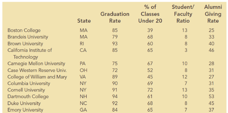
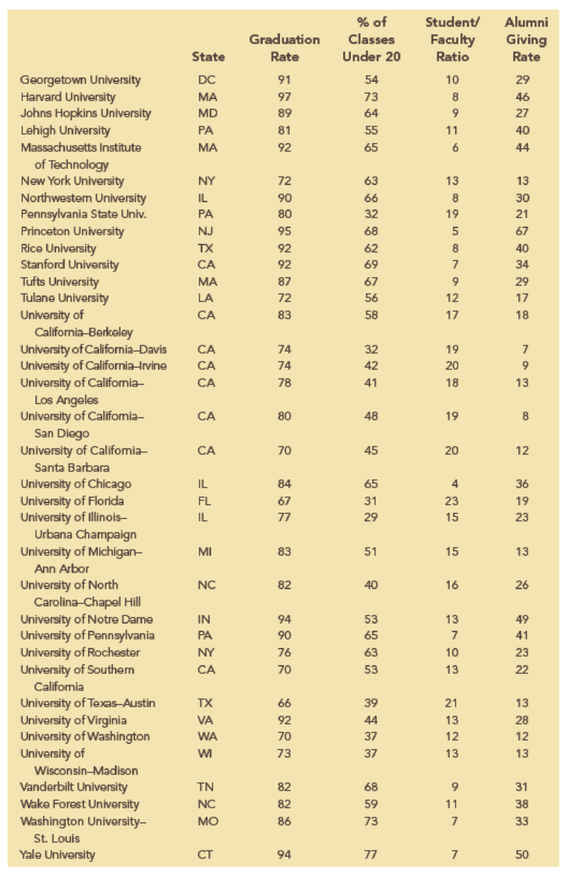
Alumni donations are an important source of revenue for colleges and universities. If administrators could determine the factors that could lead to increases in the percentage of alumni who make a donation, they might be able to implement policies that could lead to increased revenues. Research shows that students who are more satisfied with their contact with teachers are more likely to graduate. As a result, one might suspect that smaller class sizes and lower student/faculty ratios might lead to a higher percentage of satisfied graduates, which in turn might lead to increases in the percentage of alumni who make a donation. The following table shows data for 48 national universities. The Graduation Rate column is the percentage of students who initially enrolled at the university and graduated. The % of Classes Under 20 column shows the percentages of classes with fewer than 20 students that are offered. The Student/Faculty Ratio column is the number of students enrolled divided by the total number of faculty. Finally, the Alumni Giving Rate column is the percentage of alumni who made a donation to the university.

Managerial Report

1. 1. Use methods of descriptive statistics to summarize the data.
2. 2. Develop an estimated simple linear regression model that can be used to predict the alumni giving rate, given the graduation rate. Discuss your findings.
3. 3. Develop an estimated multiple linear regression model that could be used to predict the alumni giving rate using the Graduation Rate, % of Classes Under 20, and Student/Faculty Ratio as independent variables. Discuss your findings.
4. 4. Based on the results in parts (2) and (3), do you believe another regression model may be more appropriate? Estimate this model, and discuss your results.
5. 5. What conclusions and recommendations can you derive from your analysis? What universities are achieving a substantially higher alumni giving rate than would be expected, given their Graduation Rate, % of Classes Under 20, and Student/Faculty Ratio? What universities are achieving a substantially lower alumni giving rate than would be expected, given their Graduation Rate, % of Classes Under 20, and Student/Faculty Ratio? What other independent variables could be included in the model?

To determine

Summarize the data using the methods of descriptive statistics.

Answer to Problem 1C

The numerical summaries of the data are as follows:

Explanation of Solution

Calculation:

The data is related to the Alumni Giving Rate for 48 national universities.

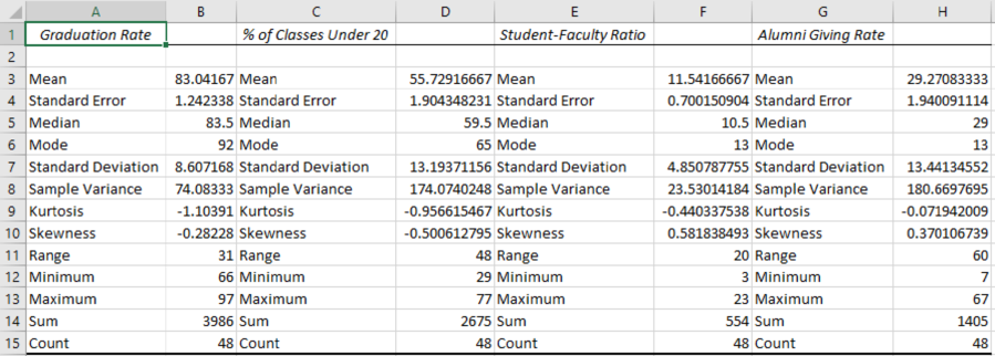
Descriptive Statistics:

Step-by-step procedure to get the descriptive statistics using EXCEL software:

• Open an EXCEL sheet named as AlumnniGiving.
• Select Data > Data Analysis > Descriptive Statistics.
• Click OK.
• Under Input Range, enter $C$1:$F$49.
• Choose Grouped By as Columns.
• Select Labels in the first row.
• Select Summary statistics.
• Under Output Range, enter $J$1.
• Click OK.

Output obtained using EXCEL software is given below:

According to the output, it is found that mean, standard deviation, and median of the Graduate Rate are 83.042, 8.61, and 83.5, respectively.

The mean, standard deviation, and median of % of classes Under 20 are 55.73, 13.19, and 59.5, respectively.

The mean, standard deviation, and median for the Student–Faculty Ratio are 11.54, 4.85, and 10.5, respectively.

Step-by-step procedure to obtain the correlation coefficient using EXCEL software:

• Select Data > Data Analysis > Descriptive Statistics.
• Click OK.
• Under Input Range, enter $C$1:$F$49.
• Choose Grouped By as Columns.
• Select Labels in the first row.
• Click Ok.

Output obtained using the EXCEL software is given below:

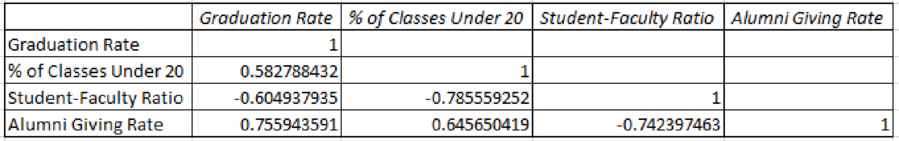
On observing the output of the correlation, it is clear that the graduate rate is positively related with the % of class under 20 and the Alumni Giving Rate and the graduate rate are negatively related with the Student–Faculty Ratio. The % of classes Under 30 is negatively related with the Student–Faculty Ratio and the % of classes Under 20 is positively related with the Alumni Giving Ratio. Finally, the Student–Faculty Ratio is negatively related to the Alumni Giving Rate.

To determine

Obtain the estimated simple linear regression model that can be used to predict the alumni-giving rate, given the graduation rate and provide comments about the findings.

Answer to Problem 1C

The estimated regression equation that could be used to predict t, the alumni-giving rateis $\underset{\_}{\widehat{y}=-68.76+1.18x}$.

Explanation of Solution

Calculation:

In this situation, the Graduation rateis the independent variable $\left(x\right)$ and the Alumni-Giving Rate is the dependent variable (y).

Regression of the Alumni-giving rate using the Graduation rate:

Step-by-step procedure to obtain the regression equation using EXCEL software:

• Select Data>Data Analysis>Regression.
• Click OK.
• Under Input Y Range, enter $F$1:$F$49.
• Under Input X Range, enter $C$1:$C$49.
• Click the box of Labels.
• Under New Worksheet.
• Click OK.

Output obtained using EXCEL software is given as follows:

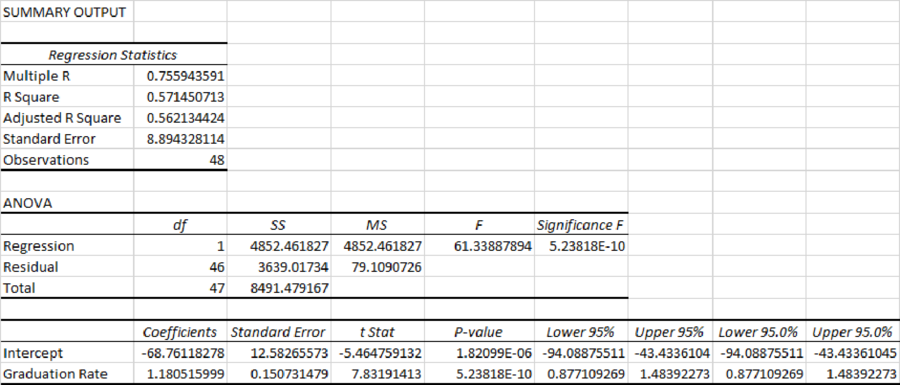
Thus, the estimated regression equation that could be used to predict the alumni-giving rate, given the graduation rate is $\widehat{y}=-68.76+1.18x$.

From the output, the slope, b=1.18, which is positive. The positive value of slope depicts that the alumni giving rate is expected to increase or decrease by 1.18 percentage as the graduation rate increases or decreases by one.

R² (R-squared):

The coefficient of determination (R²) is defined as the proportion of variation in the observed values of the response variable that is explained by the regression. The squared correlation gives the fraction of variability of the response variable (y) accounted for by the linear regression model.

From the output, R square=57.15%.

Thus, only 57.15% variability in the alumni-giving rateis explained by the variability in the graduation rate.

To determine

Create an estimated multiple linear regression model that could be used to predict the alumni-given rate using the Graduation Rate, % of Classes Under 20, and Student/Faculty Ratio as independent variables and provide the comments about the findings.

Answer to Problem 1C

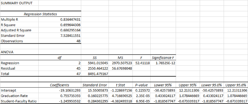
The estimated multiple linear regression model that could be used to predict the alumni-given rate using the Graduation Rate, % of Classes Under 20, and Student/Faculty Ratio as independent variables is $\widehat{y}=-20.72+0.748x_1+0.029x_2-1.19x_3$.

Explanation of Solution

Calculation:

In this given problem, the Graduation rate $\left(x_1\right)$, % of Classes Under 20$\left(x_2\right)$, and Student/Faculty Ratio $\left(x_3\right)$ are the independent variables and the Alumni-giving rate is the dependent variable (y)

Step-by-step procedure to obtain the estimated regression equation using EXCEL:

• In Data, select Data Analysis and choose Regression.
• In Input Y Range, select $F$1:$F$49.
• In Input X Range, select $C$1:$E$49.
• Select Labels.
• Click on Confidence Levels and type 95.
• Select the Residuals plot check box.
• Click OK.

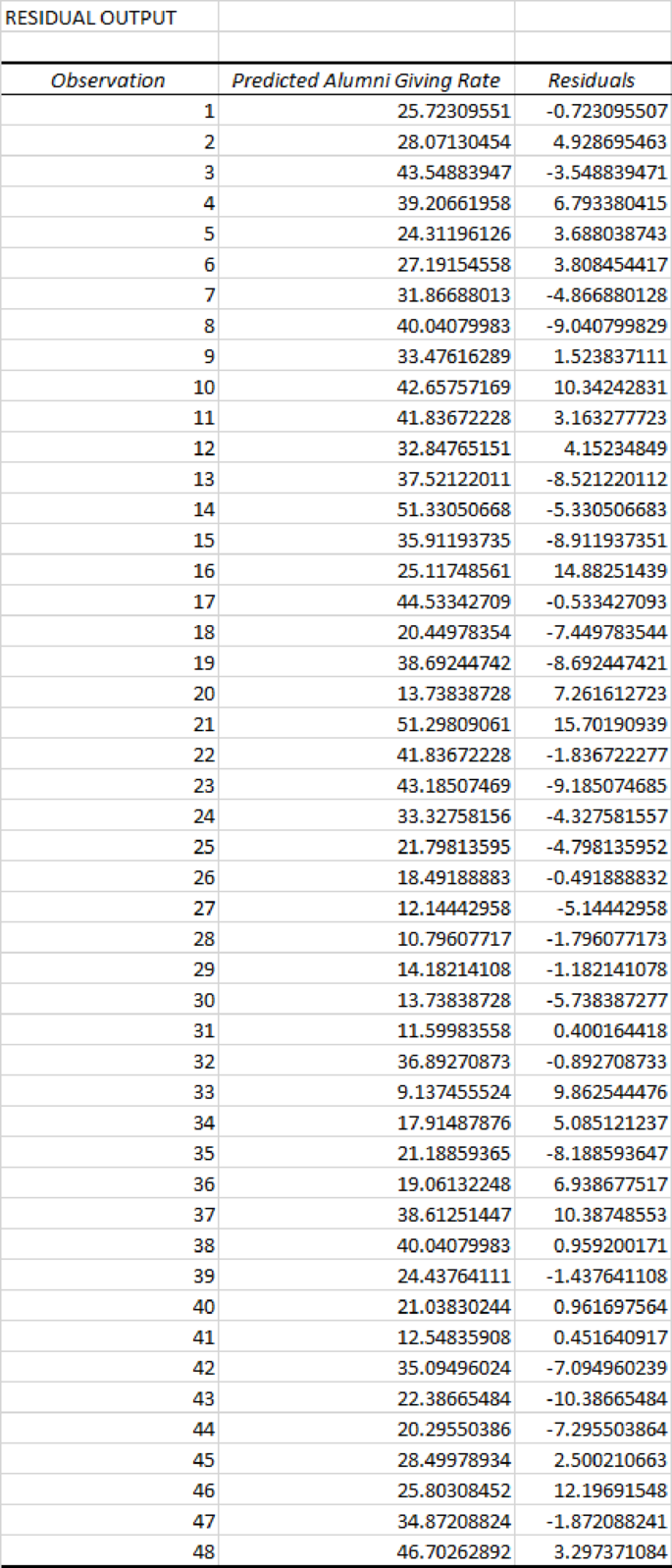
Output obtained using EXCEL is given below:

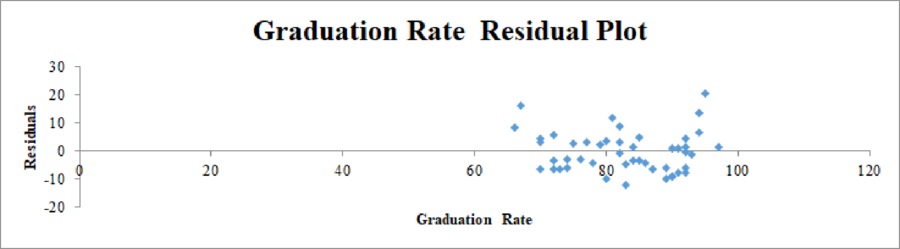
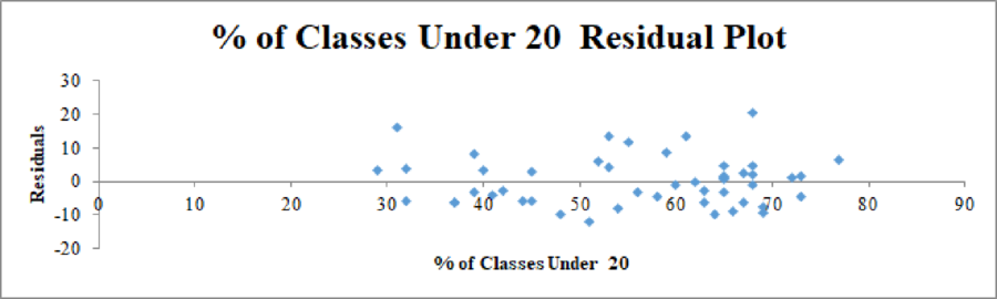
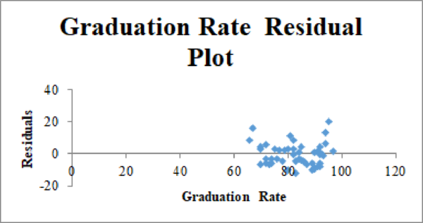
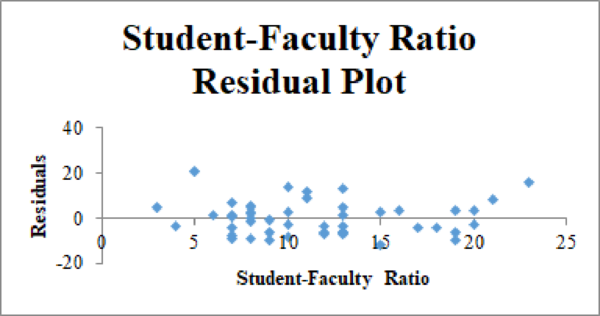
Residual plot for Graduation Rate and % of Classes Under 20:

Thus, the estimated multiple linear regression model that could be used to predict the alumni-given rate using the Graduation Rate, % of Classes Under 20, and Student/Faculty Ratio as independent variables is $\widehat{y}=-20.72+0.748x_1+0.029x_2-1.19x_3$.

Graduation Rate:

From the output, the slope, $b_1=0.748$, which is positive. The positive value of slope depicts that the alumni-giving rate is expected to increase or decrease by 1.18 percentage as the graduation rate increases or decreases by one.

% of classes Under 20:

From the output, the slope, $b_2=0.029$, which is positive. The positive value of slope depicts that the alumni-giving rate is expected to increase or decrease by 0.029 percentage as % of classes under 20 increases or decreases by one.

Student–Faculty Ratio:

From the output, the slope, $b_3=-1.19$, which is negative. The negative value of slope depicts that the alumni-giving rate is expected to decrease or increase by 1.19 percentage as the student–faculty ratio decreases or increases by one.

R² (R-squared):

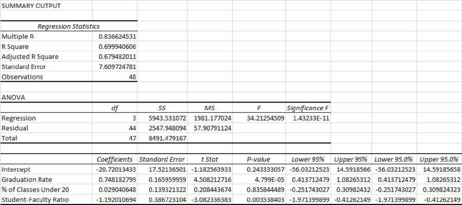
From the output, R square=69.99%.

Thus, only 69.99% variability in the alumni-giving rate (response variable) is explained by the explanatory variables in the regression equation.

To determine

State whether it is believed that another regression model may be more appropriate, if so, estimate the model and discuss the findings.

Answer to Problem 1C

The estimated multiple linear regression model that could be used to predict the alumni-given rate using the Graduation Rate and Student/Faculty Ratio as independent variables is $\widehat{y}=-19.11+0.756x_1-1.246x_2$.

The second-order quadratic model is $\underset{\_}{\widehat{y}=294.33-6.92x_1+0.047x_1^2-1.35x_2}$.

Explanation of Solution

Calculation:

For Graduation rate:

Consider that ${\beta }_1$ is the slope of the regression equation corresponding to the graduation rate.

Null hypothesis:

$H_0:{\beta }_1=0$

That is, there is no significant relationship between the Alumni giving rate and graduation rate.

Alternative hypothesis:

$H_a:{\beta }_1\ne 0$

That is, there is a significant relationship between the Alumni giving rate and graduation rate.

From the output in Part (3), it is found that the t-test statistic corresponding to comfort is 4.51 with p value of approximately 0.00005.

Level of significance:

The assumed level of significance is $\alpha =0.05$.

Conclusion:

Here, the p value is less than the level of significance.

That is, $p\text{value}\left(=0.00005\right)<\alpha \left(=0.05\right)$

Thus, the decision is “reject the null hypothesis”.

Therefore, the data provide sufficient evidence to conclude that there is a significant relationship between the Alumni-giving rate and graduation rate at 0.05 level of significance.

For % of classes under 20:

Consider that ${\beta }_2$ is the slope of the regression equation corresponding to “% of classes under 20”.

Null hypothesis:

$H_0:{\beta }_2=0$

That is, there is no significant relationship between the alumni-giving rate and % of classes under 20.

Alternative hypothesis:

$H_a:{\beta }_2\ne 0$

That is, there is a significant relationship between the alumni-giving rate and % of classes under 20.

From the output in Part (a), it is found that the t-test statistic corresponding to % of classes under 20 is 0.2084 with p value of approximately 0.8358.

Conclusion:

Here, the p value is greater than the level of significance.

That is, $p\text{value}\left(=0.8358\right)>\alpha \left(=0.05\right)$

Thus, the decision is “fail to reject the null hypothesis”.

Therefore, the data do not provide sufficient evidence to conclude that there is a significant relationship between the alumni-giving rate and % of classes under 20 at 0.05 level of significance.

For Student–Faculty Ratio:

Consider that ${\beta }_3$ is the slope of the regression equation corresponding to the student–faculty ratio.

Null hypothesis:

$H_0:{\beta }_3=0$

That is, there is no significant relationship between the alumni-giving rate and student faculty ratio.

Alternative hypothesis:

$H_a:{\beta }_3\ne 0$

That is, there is a significant relationship between the alumni-giving rate and student faculty ratio.

From the output in Part (a), it is found that the t-test statistic corresponding to in-house dining is -3.082 with p value of approximately 0.0035.

Conclusion:

Here, the p value is less than the level of significance.

That is, $p\text{value}\left(=0.0035\right)<\alpha \left(=0.05\right)$

Thus, the decision is “reject the null hypothesis”.

Therefore, the data provide sufficient evidence to conclude that there is a significant relationship between the alumni-giving rate and student faculty ratio at 0.01 level of significance.

Now, by comparing the results based on the p-value, it is clear that “% of class under 20” in the regression model in not a good predictor.

In this situation, remove “% of class under 20” variable from the model and rerun the test by considering “Graduation rate” and “student faculty ratio” as the explanatory variable and the “alumni-giving rate” as the response variable.

The estimated regression model will be as given below:

In this given problem, the Graduation rate $\left(x_1\right)$ and Student/Faculty Ratio $\left(x_2\right)$ are the independent variables and the Alumni-giving rate is the dependent variable (y)

Step-by-step procedure to obtain the estimated regression equation using EXCEL:

• In Data, select Data Analysis and choose Regression.
• In Input Y Range, select $F$1:$F$49.
• In Input X Range, select $D$1:$E$49.
• Select Labels.
• Click on Confidence Levels and type 95.
• Select the Residuals plot check box.
• Click OK.

Output obtained using EXCEL is given below:

Residual plot for the Graduation Rate and Student–Faculty Ratio:

Thus, the estimated multiple linear regression model that could be used to predict the alumni-given rate using the Graduation Rate and Student/Faculty Ratio as independent variables is $\widehat{y}=-19.11+0.756x_1-1.246x_2$.

Graduation Rate:

From the output, the slope, $b_1=0.756$, which is positive. The positive value of slope depicts that the alumni-giving rate is expected to increase or decrease by 1.18 percentage as the graduation rate increases or decreases by one.

Student–Faculty Ratio:

From the output, the slope, $b_3=-1.246$, which is negative. The negative value of slope depicts that the alumni-giving rate is expected to decrease or increase by 1.246 percentage as the student–faculty ratio decreases or increases by one.

R² (R-squared):

From the output, R square=69.96%.

Thus, only 69.96% variability in the alumni-giving rate (response variable) is explained by the explanatory variables in the regression equation.

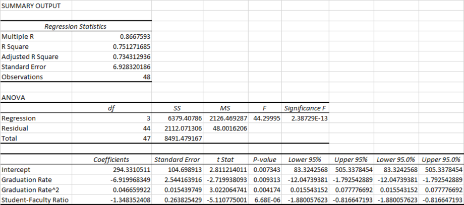
Based on output, it is observed that the R-squared value decreases by 0.04% after removing the % of class under 20 from the dataset, which indicates that the relationship between the alumni-giving rate and the graduation rate may be non-linear. Therefore, it is appropriate to estimate the second-order quadratic relationship between the two variables.

The second-order quadratic model will be as given below:

$\widehat{y}=b_0+b_1{x}_1+b_2{x}_1^2+b_3{x}_2$

Step-by-step procedure to obtain the second-order quadratic regression equation using EXCEL:

• Insert a new column “Graduate Rate^2” in between C and D.
• In cell D, Enter “=C2^2”.
• Drag the cursor till the end of the dataset.
• In Data, select Data Analysis and choose Regression.
• In Input Y Range, select $F$1:$F$49.
• In Input X Range, select $C$1:$E$49.
• Select Labels.
• Click on Confidence Levels and type 95.
• Select the Residuals plot check box.
• Click OK.

Output obtained using EXCEL is given below:

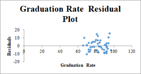
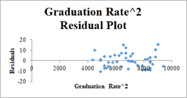
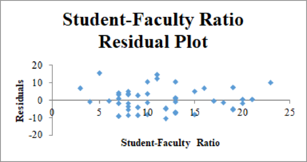
Residual plot for the Graduation Rate, Graduation Rate^2, and Student–Faculty Ratio:

The second-order quadratic model is as follows:

$\underset{\_}{\widehat{y}=294.33-6.92x_1+0.047x_1^2-1.35x_2}$

R²(R-squared):

From the output, R square=75.13%.

Thus, only 75.13% variability in the alumni-giving rate (response variable) is explained by the explanatory variables in the regression equation.

To determine

Discuss about the universities that are achieving a substantially higher alumni-giving rate than the expected, given that the graduation rate, % of classes under 20, and student/faculty ratio.

Discuss about the universities that are achieving a substantially loweralumni-giving rate than the expected, given that the graduation rate, % of classes under 20, and student/faculty ratio.

Also explain the other independent variables that could be included in the model.

Explanation of Solution

Using the output corresponding to the second-order quadratic model, the residual explain about the predicts the universities that are achieving a substantially higher and loweralumni giving rate and is given as below:

On observing the results of residual, the Alumni-giving rate at the Wake Forest University, U. of Florida, Dartmouth College, Lehigh University, U. of Notre Dame, Princeton University is approximately greater than 9% from the model predicts. Therefore, the presidents of those Universities will be glad with the determinations of the offices of Alumni Affairs.

Also, the results of residual reveal that the Alumni-giving rate at U. of Washington, Georgetown University, Columbia University, Johns Hopkins University, Stanford University,and North-western University, U. of Michigan–Ann Arbor is below 8% from the predicted model. Therefore, the presidents of those Universities will be suggested to do hard work with the determinations of the offices of Alumni Affairs.