
Videos
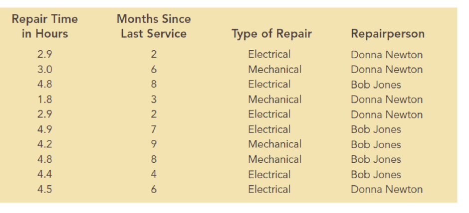
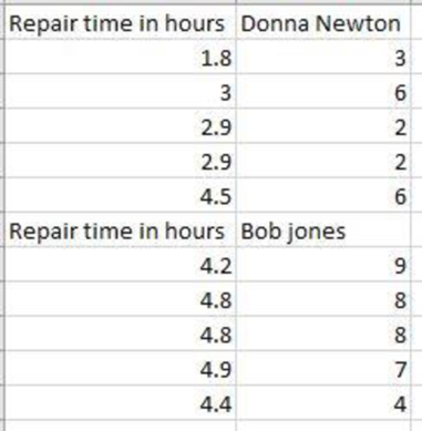
Johnson Filtration. Inc., provides maintenance service for water filtration systems throughout southern Florida. Customers contact Johnson with requests for maintenance service on their water filtration systems. To estimate the service time and the service cost. Johnson’s managers want to predict the repair time necessary for each maintenance request. Hence, repair time in hours is the dependent variable. Repair time is believed to be related to three factors: the number of months since the last maintenance service, the type of repair problem (mechanical or electrical), and the repairperson who performs the repair (Donna Newton or Bob Jones). Data for a sample of 10 service calls are reported in the following table:
- a. Develop the simple linear regression equation to predict repair time given the number of months since the last maintenance service, and use the results to test the hypothesis that no relationship exists between repair time and the number of months since the last maintenance service at the 0.05 level of significance. What is the interpretation of this relationship? What does the coefficient of determination tell you about this model?
- b. Using the simple linear regression model developed in part (a), calculate the predicted repair time and residual for each of the 10 repairs in the data. Sort the data in ascending order by value of the residual. Do you see any pattern in the residuals for the two types of repair? Do you see any pattern in the residuals for the two repairpersons? Do these results suggest any potential modifications to your simple linear regression model? Now create a scatter chart with months since last service on the x-axis and repair time in hours on the y-axis for which the points representing electrical and mechanical repairs are shown in different shapes and/or colors. Create a similar scatter chart of months since last service and repair time in hours for which the points representing repairs by Bob Jones and Donna Newton are shown in different shapes and/or colors. Do these charts and the results of your residual analysis suggest the same potential modifications to your simple linear regression model?
- c. Create a new dummy variable that is equal to zero if the type of repair is mechanical and one if the type of repair is electrical. Develop the multiple regression equation to predict repair time, given the number of months since the last maintenance service and the type of repair. What are the interpretations of the estimated regression parameters? What does the coefficient of determination tell you about this model?
- d. Create a new dummy variable that is equal to zero if the repairperson is Bob Jones and one if the repairperson is Donna Newton. Develop the multiple regression equation to predict repair time, given the number of months since the last maintenance service and the repairperson. What are the interpretations of the estimated regression parameters? What does the coefficient of determination tell you about this model?
- e. Develop the multiple regression equation to predict repair time, given the number of months since the last maintenance service, the type of repair, and the repairperson. What are the interpretations of the estimated regression parameters? What does the coefficient of determination tell you about this model?
- f. Which of these models would you use? Why?
a.
Find an estimated regression equation that could be used to predict the repair time, given the number of months since the last maintenance service.
Test whether there is any relationship between the repair time and the number of months since the last maintenance service using the level of significance of 0.05. Interpret the test results.
Interpret the value of coefficient of determination.
Answer to Problem 13P
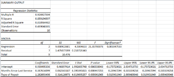
The estimated regression equation that could be used to predict the repair time, given the number of months since the last maintenance service, is
There is sufficient evidence to conclude that there is a linear relationship between the repair time and the number of months since the last maintenance service.
The amount of variation explained in the repair time by the number of months since the last maintenance service is 53.42%.
Explanation of Solution
Calculation:
Here, the repair time is the dependent variable, and the number of months since the last maintenance service is the independent variable.
Step-by-step procedure to obtain the estimated regression equation using EXCEL is defined as follows:
- In EXCEL sheet, enter Repair time in Hours and Months since the last service in columns A and B, respectively.
- In Data, select Data Analysis and choose Regression.
- In Input Y Range, select $A$1:$A$11.
- In Input X Range, select $B$1:$B$11.
- Select Labels.
- Click OK.
Output obtained using EXCEL is given below:
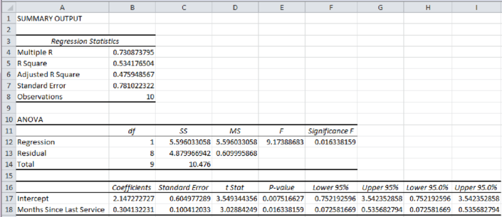
Thus, the estimated regression equation that could be used to predict the repair time, given the number of months since the last maintenance service, is
The null and alternative hypotheses to test whether there is a relationship between repair time and the number of months since the last maintenance service are given as follows:
It is given that the level of significance is 0.05.
From the above output, the P-value is 0.0163.
Decision rule:
The null hypothesis is rejected if the P-value is less than or equal to the level of significance. Otherwise, do not reject the null hypothesis.
Here, the P-value of 0.0163 is less than the level of significance (0.05). Hence, the null hypothesis is rejected.
Therefore, there is sufficient evidence to conclude that there is a linear relationship between the repair time and the number of months since the last maintenance service.
Coefficient of determination:
The coefficient of determination (R-square) value explains the percentage of variation explained in the dependent variable by the independent variables.
From the given output, the value of R-square is approximately 0.5342. That is, the amount of variation explained in the repair time by the number of months since the last maintenance service is 53.42%.
b.
Find the predicted repair time and residual for each of the 10 repairs.
Arrange the data in the ascending order by value of the residual. Is there any pattern observed in the residuals in the two types of repairs. Is there any pattern observed in the residuals in the two repairpersons. Explain whether these results suggest any modifications to the obtained regression model.
Construct a scatterplot with months since the last maintenance service on the x-axis and repair time on the y-axis and differentiate the points between two types of repairs.
Construct a scatterplot with months since the last maintenance service on the x-axis and repair time on the y-axis and differentiate the points between two types of repair persons.
Explain whether these results suggest any modifications to the obtained regression model.
Answer to Problem 13P
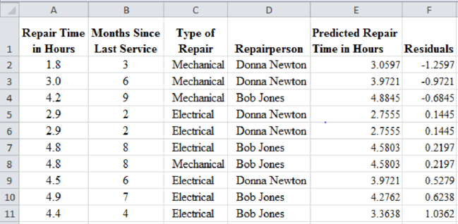
The predicted and residual values for all the observations are calculated and given in ascending order by residuals as follows:
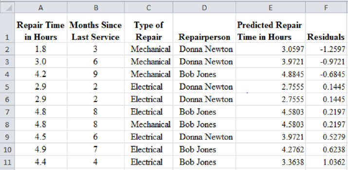
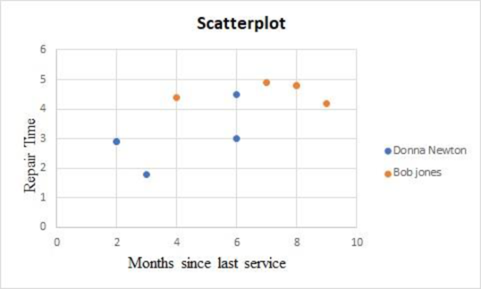
From the above result, mechanical repairs are generally negative residual values and electrical repairs have positive residual values. That is, the mechanical repairs take less time when compared to electrical repairs.
The first two large negative residuals are made by Donna Newton. The residuals of Bob Jones are positive. That is, the repairs by Bob Jones take more time than the predicted values.
The scatterplots obtained using EXCEL are given below:
The above results suggest including these categorical variables into the regression model by creating dummy variables.
Explanation of Solution
Calculation:
From the given dataset, the first observation of Months since last service is 2.
The predicted repair time for the first observation is calculated as follows:
Thus, the predicted repair time is 2.7555 hours.
The observed repair time for the first observation is given as 2.9 hours.
The residual of the first observation is calculated as follows:
Similarly, the predicted and residual values for all the observations are calculated and given in the ascending order by residuals as follows:
From the above result, mechanical repairs are generally negative residual values and electrical repairs have positive residual values. That is, the mechanical repairs take less time when compared to electrical repairs.
The first two large negative residuals are made by Donna Newton. The residuals of Bob Jones are positive. That is, the repairs by Bob Jones take more time than the predicted values.
The above results suggest including these categorical variables into the regression model by creating dummy variables.
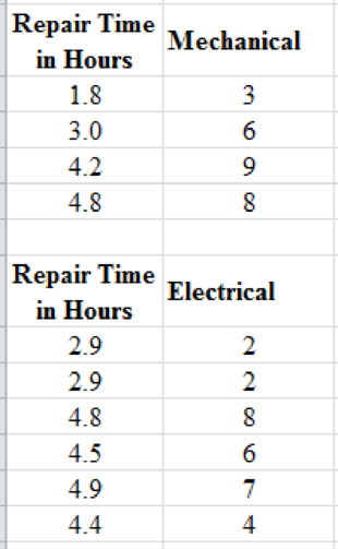
Separate the above data into two tables with respect to the type of repair considering months since last service as follows:
Step-by-step procedure to obtain the scatterplot using EXCEL is given as follows:
- Select the first data with labels.
- Go to Insert, select Charts and select Scatterplot.
- A scatterplot will be displayed.
- Select and copy the second data with labels.
- Click on the scatterplot and click on Paste.
- Select Paste special.
- Select New series and Columns.
- Select Series names in first row and Categories (X values) in first column.
- Click OK.
Output obtained using EXCEL is given below:
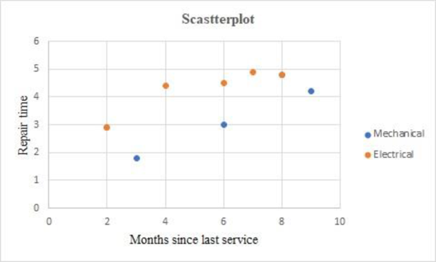
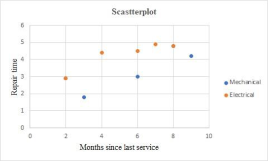
The above chart indicates that the electrical repairs take more time than mechanical repairs.
Separate the above data into two tables with respect to repair person considering months since last service as follows:
Step-by-step procedure to obtain the scatterplot using EXCEL is given as follows:
- Select the first data with labels.
- Go to Insert, select Charts and select Scatterplot.
- A scatterplot will be displayed.
- Select and copy the second data with labels.
- Click on the scatterplot and click on Paste.
- Select Paste special.
- Select New series and Columns.
- Select Series names in first row and Categories (X values) in first column.
- Click OK.
Output obtained using EXCEL is given below:

The above chart indicates that the repairs by Bob Jones take more time than Donna Newton.
The above two scatterplots suggest including these categorical variables into the regression model by creating dummy variables.
c.
Find an estimated regression equation that could be used to predict the repair time, given the number of months since the last maintenance service and the type of repair.
Interpret the value of coefficient of determination.
Answer to Problem 13P
The estimated regression equation that could be used to predict the repair time, given the number of months since the last maintenance service and the type of repair, is as follows:
It increases every month since the last service will increase the repair time by 0.3876 hours.
The repair time of mechanical repairs is 1.2627 hours less than the repair time of electrical repairs.
The amount of variation explained in the repair time by the number of months since the last maintenance service and the type of repair is 85.92%.
Explanation of Solution
Calculation:
Here, the repair time is the dependent variable. The number of months since the last maintenance service and the type of repair are the independent variables.
Step-by-step procedure to obtain the estimated regression equation using EXCEL is defined as follows:
- Create a variable type of repair.
- In the variable type of repair, enter 0 of the repair is mechanical and enter 1 if the repair is electrical.
- In Data, select Data Analysis and choose Regression.
- In Input Y Range, select $A$1:$A$11.
- In Input X Range, select $B$1:$C$11.
- Select Labels.
- Click OK.
Output obtained using EXCEL is given below:
Thus, the estimated regression equation that could be used to predict the repair time, given the number of months since the last maintenance service and the type of repair is as follows:
Interpretation of parameters:
It increases every month since the last service will increase the repair time by 0.3876 hours.
The repair time of mechanical repairs is 1.2627 hours less than the repair time of electrical repairs.
From the given output, the value of R-square is approximately 0.8592. That is, the amount of variation explained in the repair time by the number of months since the last maintenance service and the type of repair is 85.92%.
d.
Find an estimated regression equation that could be used to predict the repair time, given the number of months since the last maintenance service and the repair person.
Interpret the value of coefficient of determination.
Answer to Problem 13P
The estimated regression equation that could be used to predict the repair time, given the number of months since the last maintenance service and the repair person, is as follows:
It increases every month since the last service will increase the repair time by 0.1519 hours.
The repair time of Bob Jones is 1.0835 hours more than the repair time of Donna Newton.
From the given output, the value of R-square is approximately 0.6805. That is, the amount of variation explained in the repair time by the number of months since the last maintenance service and the repairperson is 68.05%.
Explanation of Solution
Calculation:
Here, the repair time is the dependent variable. The number of months since the last maintenance service and the repair person are the independent variables.
Step-by-step procedure to obtain the estimated regression equation using EXCEL is defined as follows:
- Create a variable type of repair.
- In the variable type of repair, enter 0 of the repairperson is Bob Jones and enter 1 if the repairperson is Donna Newton.
- Place the variables repair time, number of months since the last maintenance service, and the repairperson in the columns A, B, and C, respectively.
- In Data, select Data Analysis and choose Regression.
- In Input Y Range, select $A$1:$A$11.
- In Input X Range, select $B$1:$C$11.
- Select Labels.
- Click OK.
Output obtained using EXCEL is given below:
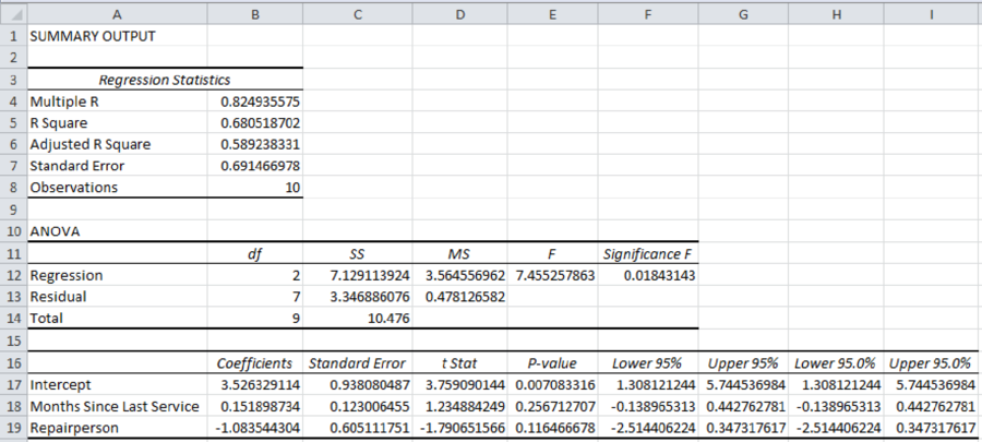
Thus, the estimated regression equation that could be used to predict the repair time, given the number of months since the last maintenance service and the repairperson, is as follows:
Interpretation of parameters:
It increases every month since the last service will increase the repair time by 0.1519 hours.
The repair time of Bob Jones is 1.0835 hours more than the repair time of Donna Newton.
From the given output, the value of R-square is approximately 0.6805. That is, the amount of variation explained in the repair time by the number of months since the last maintenance service and the repairperson is 68.05%.
e.
Find an estimated regression equation that could be used to predict the repair time, given the number of months since the last maintenance service, the type of repair, and the repair person.
Interpret the value of coefficient of determination.
Answer to Problem 13P
The estimated regression equation that could be used to predict the repair time, given the number of months since the last maintenance service, the type of repair, and the repair person is as follows:
It increases every month since the last service will increase the repair time by 0.2914 hours.
The repair time of mechanical repairs is 1.1024 hours less than the repair time of electrical repairs.
The repair time of Bob Jones is 0.6091 hours more than the repair time of Donna Newton.
From the given output, the value of R-square is approximately 0.9002. That is, the amount of variation explained in the repair time by the number of months since the last maintenance service and the repair person is 90.02%.
Explanation of Solution
Calculation:
Here, the repair time is the dependent variable. The number of months since the last maintenance service, the type of repair, and the repairperson are the independent variables.
Step-by-step procedure to obtain the estimated regression equation using EXCEL is defined as follows:
- Place the variables’ repair time, number of months since the last maintenance service, the type of repair, and the repair person in the columns A, B, C, and D, respectively.
- In Data, select Data Analysis and choose Regression.
- In Input Y Range, select $A$1:$A$11.
- In Input X Range, select $B$1:$D$11.
- Select Labels.
- Click OK.
Output obtained using EXCEL is given below:
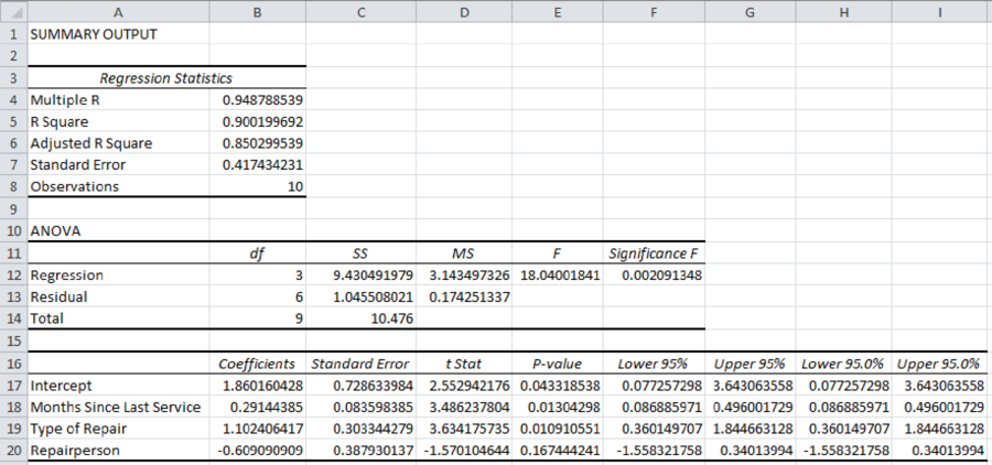
Thus, the estimated regression equation that could be used to predict the repair time, given the number of months since the last maintenance service, the type of repair, and the repair person is as follows:
Interpretation of parameters:
It increases every month since the last service will increase the repair time by 0.2914 hours.
The repair time of mechanical repairs is 1.1024 hours less than the repair time of electrical repairs.
The repair time of Bob Jones is 0.6091 hours more than the repair time of Donna Newton.
From the given output, the value of R-square is approximately 0.9002. That is, the amount of variation explained in the repair time by the number of months since the last maintenance service and the repair person is 90.02%.
f.
Identify the best regression model among the models.
Answer to Problem 13P
The preferable model is the regression model in Part (c).
Explanation of Solution
The R-square value of the regression model in Part (a) is 0.5341. Here, the only independent variable is the number of months since the last maintenance service. Here, the independent variable is significant.
The R-square value of the regression model in Part (c) is 0.8592. Here, the independent variables are the number of months since the last maintenance service and the type of repair. Here, both the independent variables are significant.
The R-square value of the regression model in Part (d) is 0.6805. Here, the independent variables are the number of months since the last maintenance service and the repair person. Here, both the independent variables are insignificant.
The R-square value of the regression model in Part (e) is 0.9002. Here, the independent variables are the number of months since the last maintenance service, the type of repair, and the repair person. Here, the independent variable repair person is insignificant. The value of R-square from the model in Part (c) is increased due to the multicollinearity between the variables such as the number of months since the last maintenance service and the repair person.
The best regression model is always a model with less number of independent variables that are significant and higher value of R-square.
Hence, the preferable model is the regression model in Part (c).
Want to see more full solutions like this?
Chapter 7 Solutions
Essentials of Business Analytics (MindTap Course List)


- Suppose that the chance that an elementary student eats hot lunch is 30 percent. What’s the chance that, among 20 randomly selected students, between 6 and 8 students eat hot lunch (inclusive)?arrow_forwardBob’s commuting times to work are varied. He makes it to work on time 80 percent of the time. On 12 randomly selected trips to work, what’s the chance that Bob makes it on time at least 10 times?arrow_forwardYour chance of winning a small prize in a scratch-off ticket is 10 percent. You buy five tickets. What’s the chance you will win at least one prize?arrow_forward
- Suppose that 60 percent of families own a pet. You randomly sample four families. What is the chance that two or three of them own a pet?arrow_forwardIf 40 percent of university students purchase their textbooks online, in a random sample of five students, what’s the chance that exactly one of them purchased their textbooks online?arrow_forwardA stoplight is green 40 percent of the time. If you stop at this light eight random times, what is the chance that it’s green exactly five times?arrow_forward
- If 10 percent of the parts made by a certain company are defective and have to be remade, what is the chance that a random sample of four parts has one that is defective?arrow_forwardQuestion 4 Fourteen individuals were given a complex puzzle to complete. The times in seconds was recorded for their first and second attempts and the results provided below: 1 2 3 first attempt 172 255 second attempt 70 4 5 114 248 218 194 270 267 66 6 7 230 219 341 174 8 10 9 210 261 347 218 200 281 199 308 268 243 236 300 11 12 13 14 140 302 a. Calculate a 95% confidence interval for the mean time taken by each individual to complete the (i) first attempt and (ii) second attempt. [la] b. Test the hypothesis that the difference between the two mean times for both is 100 seconds. Use the 5% level of significance. c. Subsequently, it was learnt that the times for the second attempt were incorrecly recorded and that each of the values is 50 seconds too large. What, if any, difference does this make to the results of the test done in part (b)? Show all steps for the hypothesis testarrow_forwardQuestion 3 3200 students were asked about the importance of study groups in successfully completing their courses. They were asked to provide their current majors as well as their opinion. The results are given below: Major Opinion Psychology Sociology Economics Statistics Accounting Total Agree 144 183 201 271 251 1050 Disagree 230 233 254 227 218 1162 Impartial 201 181 196 234 176 988 Total 575 597 651 732 645 3200 a. State both the null and alternative hypotheses. b. Provide the decision rule for making this decision. Use an alpha level of 5%. c. Show all of the work necessary to calculate the appropriate statistic. | d. What conclusion are you allowed to draw? c. Would your conclusion change at the 10% level of significance? f. Confirm test results in part (c) using JASP. Note: All JASP input files and output tables should be providedarrow_forward
- Question 1 A tech company has acknowledged the importance of having records of all meetings conducted. The meetings are very fast paced and requires equipment that is able to capture the information in the shortest possible time. There are two options, using a typewriter or a word processor. Fifteen administrative assistants are selected and the amount of typing time in hours was recorded. The results are given below: 1 2 3 4 5 6 7 8 9 10 11 12 13 14 15 typewriter 8.0 6.5 5.0 6.7 7.8 8.5 7.2 5.7 9.2 5.7 6.5 word processor 7.2 5.7 8.3 7.5 9.2 7.2 6.5 7.0 6.9 34 7.0 6.9 8.8 6.7 8.8 9.4 8.6 5.5 7.2 8.4 a. Test the hypothesis that the mean typing time in hours for typewriters is less than 7.0. Use the 1% level of significance. b. Construct a 90% confidence interval for the difference in mean typing time in hours, where a difference is equal to the typing time in hours of word processors minus typing time in hours of typewriter. c. Using the 5% significance level, determine whether there is…arrow_forwardIllustrate 2/7×4/5 using a rectangular region. Explain your work. arrow_forwardWrite three other different proportions equivalent to the following using the same values as in the given proportion 3 foot over 1 yard equals X feet over 5 yardsarrow_forward
 Glencoe Algebra 1, Student Edition, 9780079039897...AlgebraISBN:9780079039897Author:CarterPublisher:McGraw Hill
 Functions and Change: A Modeling Approach to Coll...AlgebraISBN:9781337111348Author:Bruce Crauder, Benny Evans, Alan NoellPublisher:Cengage Learning
 Holt Mcdougal Larson Pre-algebra: Student Edition...AlgebraISBN:9780547587776Author:HOLT MCDOUGALPublisher:HOLT MCDOUGAL