Interpretation:
Determine the stability of the fixed point at the origin and find is there any other fixed points for the system. Depending on other parameters sketch the qualitatively different types of phase portrait.
Concept Introduction:
The parametric curves traced by solutions of a differential equation are known as trajectories.
The geometrical representation of collection of trajectories in a phase plane is called as phase portrait.
The point which satisfies the condition
Closed Orbit corresponds to periodic solution of the system i.e.
If nearby trajectories moving away from the fixed point then the point is said to be saddle point.
If the trajectories swirling around the fixed point, then it is an unstable fixed point.
If nearby trajectories moving away from the fixed point, then the point is said to be unstable fixed point.
If nearby trajectories moving towards the fixed point, then the point is said to be stable fixed point.
To check the stability of fixed point use Jacobian matrix
The point
Answer to Problem 7E
Solution:
The stability of the origin depends upon the values of the various parameters.
The other fixed points for the system are
The different qualitatively phase portrait are shown below.
Explanation of Solution
a)
The given system equations are
Fordetermining the stability of fixed point
Use the Jacobian matrix
The expression of the Jacobian matrix is
Substitute the expressions of
The above Jacobian matrix at the origin becomes,
The eigenvalues of the above Jacobian matrix are
From the above expressions of eigenvalues, the origin is unstable, if
And the origin is stable point if
Thus, the system is stable at origin the value of
(b)
To estimate the other fixed point of the system put
Putting
From the above equation, two conditions are determined.
Put
From the above equation, two conditions are determined.
Now, substituting
Thus, the one of the fixed point is
Now, substituting
Thus, the another fixed point is at
Therefore, there exists another two fixed point at
To check the stability of these points, use Jacobian matrix
Let’s check the stability of the fixed point
Substituting expression of
By substituting
The Jacobian matrix at the point
Here, the Jacobian matrixes are triangular matrix.
And
The eigenvalues of the triangular matrix are the diagonal elements.
Thus, the eigenvalues of Jacobian matrix
The stability of the fixed point
Both the eigenvalues have negative real parts. Hence the fixed point is stable.
If one of the eigenvalue has positive real part and another having negative real part, then the fixed point is saddle fixed point. If both eigenvalues have positive real part, then the fixed point is unstable.
And eigenvalues of Jacobian matrix
The stability of the fixed point
If the both the eigenvalues have negative real parts, then the fixed point is stable.
If one of the eigenvalue has positive real part and another having negative real part, then the fixed point is saddle fixed point. If both eigenvalues have positive real part, then the fixed point is unstable.
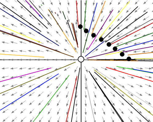
(c) The different phase portrait for the different value of the parameter constant is plotted as:
Considering a constant parameter is as follows:
The phase portrait for the above constant value is plotted as follows:
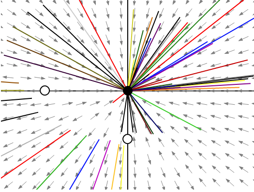
This phase portrait describes that
Considering a constant parameter is as follows:
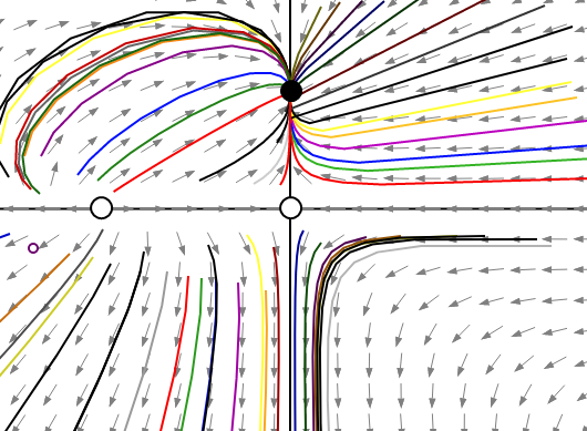
This phase portrait describes that stable point is on the
Considering a constant parameter is as follows:
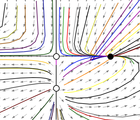
The phase portrait describes that the stable point is on
This phase portrait describes that there are infinite number of fixed points in the first quadrant of the graph and an unstable point at origin.
There are four different qualitatively phase portrait can be sketched for the system and there is no possibility of other phase portrait because the nullclines are axes and parallel lines.
Want to see more full solutions like this?
Chapter 6 Solutions
Nonlinear Dynamics and Chaos

- Let M = M₁U M₂ UM3 and K M₁ = {(x1, x2) ER²: 2 ≤ x ≤ 8, 2≤ x ≤8}, M₂ = {(x1, x2)™ € R² : 4 ≤ x₁ ≤ 6, 0 ≤ x2 ≤ 10}, M3 = {(x1, x2) Є R²: 0 ≤ x₁ ≤ 10, 4≤ x ≤ 6}, ¯ = cone {(1, 2), (1,3)†} ≤ R². (a) Determine the set E(M,K) of efficient points of M with respect to K. (b) Determine the set P(M, K) of properly efficient points of M with respect to K.arrow_forward5.17 An aluminum curtain wall panel 12 feet high is attached to large concrete columns (top and bottom) when the temperature is 65°F. No provision is made for differen- tial thermal movement vertically. Because of insulation between them, the sun heats up the wall panel to 120°F but the column to only 80°F. Determine the consequent compressive stress in the curtain wall. CONCRETE COLUMNS CONNECTIONS Stress= ALUMINUM WALL PANEL 12'-0"arrow_forward6.2 יך 4" 2" 2" Find the centroid of the following cross-sections and planes. X= Y=arrow_forward
- Find the directional derivative of the function at P in direction Varrow_forward6.4 49 Find the centroid of the following cross-sections and planes. X=_ Y= C15 XAO (CENTERED) KW14x90arrow_forward5.18 The steel rails of a continuous, straight railroad track are each 60 feet long and are laid with spaces be- tween their ends of 0.25 inch at 70°F. a. At what temperature will the rails touch end to end? b. What compressive stress will be produced in the rails if the temperature rises to 150°F? T= Stress= L= 60' 25 @T=70°Farrow_forward
- Strength of Materials Problems 5.16 A long concrete bearing wall has vertical expansion joints placed every 40 feet. Determine the required width of the gap in a joint if it is wide open at 20°F and just barely closed at 80°F. Assume α = 6 × 10⁻⁶/°F. Width= CONCRETE BEARING WALL EXPANSION JOINT 40' 40' 40' 293arrow_forwardCan you show me a step by step explanation please.arrow_forward9.7 Given the equations 0.5x₁-x2=-9.5 1.02x₁ - 2x2 = -18.8 (a) Solve graphically. (b) Compute the determinant. (c) On the basis of (a) and (b), what would you expect regarding the system's condition? (d) Solve by the elimination of unknowns. (e) Solve again, but with a modified slightly to 0.52. Interpret your results.arrow_forward
- 12.42 The steady-state distribution of temperature on a heated plate can be modeled by the Laplace equation, 0= FT T + 200°C 25°C 25°C T22 0°C T₁ T21 200°C FIGURE P12.42 75°C 75°C 00°C If the plate is represented by a series of nodes (Fig. P12.42), cen- tered finite-divided differences can be substituted for the second derivatives, which results in a system of linear algebraic equations. Use the Gauss-Seidel method to solve for the temperatures of the nodes in Fig. P12.42.arrow_forward9.22 Develop, debug, and test a program in either a high-level language or a macro language of your choice to solve a system of equations with Gauss-Jordan elimination without partial pivoting. Base the program on the pseudocode from Fig. 9.10. Test the program using the same system as in Prob. 9.18. Compute the total number of flops in your algorithm to verify Eq. 9.37. FIGURE 9.10 Pseudocode to implement the Gauss-Jordan algorithm with- out partial pivoting. SUB GaussJordan(aug, m, n, x) DOFOR k = 1, m d = aug(k, k) DOFOR j = 1, n aug(k, j) = aug(k, j)/d END DO DOFOR 1 = 1, m IF 1 % K THEN d = aug(i, k) DOFOR j = k, n aug(1, j) END DO aug(1, j) - d*aug(k, j) END IF END DO END DO DOFOR k = 1, m x(k) = aug(k, n) END DO END GaussJordanarrow_forward11.9 Recall from Prob. 10.8, that the following system of equations is designed to determine concentrations (the e's in g/m³) in a series of coupled reactors as a function of amount of mass input to each reactor (the right-hand sides are in g/day): 15c3cc33300 -3c18c26c3 = 1200 -4c₁₂+12c3 = 2400 Solve this problem with the Gauss-Seidel method to & = 5%.arrow_forward
 Trigonometry (MindTap Course List)TrigonometryISBN:9781337278461Author:Ron LarsonPublisher:Cengage Learning
 Linear Algebra: A Modern IntroductionAlgebraISBN:9781285463247Author:David PoolePublisher:Cengage Learning
 Algebra & Trigonometry with Analytic GeometryAlgebraISBN:9781133382119Author:SwokowskiPublisher:Cengage
 Mathematics For Machine TechnologyAdvanced MathISBN:9781337798310Author:Peterson, John.Publisher:Cengage Learning,