
Concept explainers
Videos
(a)
Represent this chance process with Tree diagram.
(a)
Explanation of Solution
Given information:
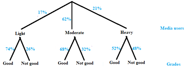
Study about media influence in young people lives aged 8 − 18:
17% were classified as light media users
62% were classified as moderate media users
21% were classified as heavy media users
Respondents with good grades:
74% light users described their grades as good
68% moderate users described their grades as good
52% heavy users described their grades as good
First level:
First level consists of three types of media users:
Light, moderate and heavy
Thus,
The first level requires three children:
Light, moderate and heavy
Second level:
In this level, there are two types of grades:
Good grades or No Good grades
Thus,
The second level consists of two children per child at the first level i.e.; Good grades or No Good grades.
The required tree diagram can be drawn as:
(b)
(b)
Answer to Problem 82E
Probability for the person with good grades is 0.6566.
Explanation of Solution
Given information:
Study about media influence in young people lives aged 8 − 18:
17% were classified as light media users
62% were classified as moderate media users
21% were classified as heavy media users
Respondents with good grades:
74% light users described their grades as good
68% moderate users described their grades as good
52% heavy users described their grades as good
Calculations:
According to the general multiplication rule,
P(A and B)=P(A∩B)=P(A)×P(B|A)=P(B)×P(A|B)
According to the
P(A∪B)=P(A or B)=P(A)+P(B)
Let
L: Light user
M: Moderate user
H: Heavy user
G: Good grades
Gc: No Good grades
Now,
The corresponding probabilities:
Probability for light user,
P(L)=0.17
Probability for moderate user,
P(M)=0.62
Probability for heavy user,
P(H)=0.21
Probability for light user with good grades,
P(G|L)=0.74
Probability for moderate user with good grades,
P(G|M)=0.68
Probability for heavy user with good grades,
P(G|H)=0.52
Apply general multiplication rule:
Probability for user with good grades and light user,
P(G and L)=P(L)×P(G|L)=0.17×0.74=0.1258
Probability for user with good grades and moderate user,
P(G and M)=P(M)×P(G|M)=0.62×0.68=0.4216
Probability for user with good grades and heavy user,
P(G and H)=P(H)×P(G|H)=0.21×0.52=0.1092
Since each person cannot become more than one type of user.
Apply the addition rule for mutually exclusive events:
P(G)=P(G and L)+P(G and M)+P(G and H) =0.1258+0.4216+0.1092 =0.6566
Thus,
Probability for the person describes his or her grades as good is 0.6566.
(c)
Conditional probability for the randomly chosen person describes his or her grade as good is a heavy user of media.
(c)
Answer to Problem 82E
Probability that the randomly chosen person describes his or her grade as good is a heavy user of media is approx. 0.1663.
Explanation of Solution
Given information:
Study about media influence in young people lives aged 8 − 18:
17% were classified as light media users
62% were classified as moderate media users
21% were classified as heavy media users
Respondents with good grades:
74% light users described their grades as good
68% moderate users described their grades as good
52% heavy users described their grades as good
Calculations:
According to the conditional probability,
P(B|A)=P(A∩B)P(A)=P(A and B)P(A)
From Part (b),
We have
Probability for the person describes his or her grades as good,
P(G)=0.6566
Probability for user with good grades and heavy user,
P(G and H)=0.1092
Apply the conditional probability:
P(H|G)=P(G and H)P(G)=0.10920.6566=78469≈0.1663
Thus,
The probability for the person describes his or her grades as good is a heavy user of media is approx. 0.1663.
Chapter 5 Solutions
EBK PRACTICE OF STAT.F/AP EXAM,UPDATED
Additional Math Textbook Solutions
Thinking Mathematically (6th Edition)
Basic Business Statistics, Student Value Edition
University Calculus: Early Transcendentals (4th Edition)
Elementary Statistics
A Problem Solving Approach To Mathematics For Elementary School Teachers (13th Edition)
A First Course in Probability (10th Edition)


- Business Discussarrow_forwardYou want to obtain a sample to estimate the proportion of a population that possess a particular genetic marker. Based on previous evidence, you believe approximately p∗=11% of the population have the genetic marker. You would like to be 90% confident that your estimate is within 0.5% of the true population proportion. How large of a sample size is required?n = (Wrong: 10,603) Do not round mid-calculation. However, you may use a critical value accurate to three decimal places.arrow_forward2. [20] Let {X1,..., Xn} be a random sample from Ber(p), where p = (0, 1). Consider two estimators of the parameter p: 1 p=X_and_p= n+2 (x+1). For each of p and p, find the bias and MSE.arrow_forward
- 1. [20] The joint PDF of RVs X and Y is given by xe-(z+y), r>0, y > 0, fx,y(x, y) = 0, otherwise. (a) Find P(0X≤1, 1arrow_forward4. [20] Let {X1,..., X} be a random sample from a continuous distribution with PDF f(x; 0) = { Axe 5 0, x > 0, otherwise. where > 0 is an unknown parameter. Let {x1,...,xn} be an observed sample. (a) Find the value of c in the PDF. (b) Find the likelihood function of 0. (c) Find the MLE, Ô, of 0. (d) Find the bias and MSE of 0.arrow_forward3. [20] Let {X1,..., Xn} be a random sample from a binomial distribution Bin(30, p), where p (0, 1) is unknown. Let {x1,...,xn} be an observed sample. (a) Find the likelihood function of p. (b) Find the MLE, p, of p. (c) Find the bias and MSE of p.arrow_forward
- Given the sample space: ΩΞ = {a,b,c,d,e,f} and events: {a,b,e,f} A = {a, b, c, d}, B = {c, d, e, f}, and C = {a, b, e, f} For parts a-c: determine the outcomes in each of the provided sets. Use proper set notation. a. (ACB) C (AN (BUC) C) U (AN (BUC)) AC UBC UCC b. C. d. If the outcomes in 2 are equally likely, calculate P(AN BNC).arrow_forwardSuppose a sample of O-rings was obtained and the wall thickness (in inches) of each was recorded. Use a normal probability plot to assess whether the sample data could have come from a population that is normally distributed. Click here to view the table of critical values for normal probability plots. Click here to view page 1 of the standard normal distribution table. Click here to view page 2 of the standard normal distribution table. 0.191 0.186 0.201 0.2005 0.203 0.210 0.234 0.248 0.260 0.273 0.281 0.290 0.305 0.310 0.308 0.311 Using the correlation coefficient of the normal probability plot, is it reasonable to conclude that the population is normally distributed? Select the correct choice below and fill in the answer boxes within your choice. (Round to three decimal places as needed.) ○ A. Yes. The correlation between the expected z-scores and the observed data, , exceeds the critical value, . Therefore, it is reasonable to conclude that the data come from a normal population. ○…arrow_forwardding question ypothesis at a=0.01 and at a = 37. Consider the following hypotheses: 20 Ho: μ=12 HA: μ12 Find the p-value for this hypothesis test based on the following sample information. a. x=11; s= 3.2; n = 36 b. x = 13; s=3.2; n = 36 C. c. d. x = 11; s= 2.8; n=36 x = 11; s= 2.8; n = 49arrow_forward
- 13. A pharmaceutical company has developed a new drug for depression. There is a concern, however, that the drug also raises the blood pressure of its users. A researcher wants to conduct a test to validate this claim. Would the manager of the pharmaceutical company be more concerned about a Type I error or a Type II error? Explain.arrow_forwardFind the z score that corresponds to the given area 30% below z.arrow_forwardFind the following probability P(z<-.24)arrow_forward
 MATLAB: An Introduction with ApplicationsStatisticsISBN:9781119256830Author:Amos GilatPublisher:John Wiley & Sons Inc
 Probability and Statistics for Engineering and th...StatisticsISBN:9781305251809Author:Jay L. DevorePublisher:Cengage Learning
 Statistics for The Behavioral Sciences (MindTap C...StatisticsISBN:9781305504912Author:Frederick J Gravetter, Larry B. WallnauPublisher:Cengage Learning
 Elementary Statistics: Picturing the World (7th E...StatisticsISBN:9780134683416Author:Ron Larson, Betsy FarberPublisher:PEARSON
 The Basic Practice of StatisticsStatisticsISBN:9781319042578Author:David S. Moore, William I. Notz, Michael A. FlignerPublisher:W. H. Freeman
 Introduction to the Practice of StatisticsStatisticsISBN:9781319013387Author:David S. Moore, George P. McCabe, Bruce A. CraigPublisher:W. H. Freeman