
Videos
Archery. An archer shoots an arrow into a square target 6 feet on a side whose center we call the origin. The outcome of this random experiment is the point in the target hit by the arrow. The archer scores 10 points if she hits the bull’s eye—a disk of radius 1 foot centered at the origin; she scores 5 points if she hits the ring with inner radius 1 foot and outer radius 2 feet centered at the origin; and she scores 0 points otherwise. Assume that the archer will actually hit the target and is equally likely to hit any portion of the target. For one arrow shot, let S be the score. A probability distribution for the random variable S is as follows.
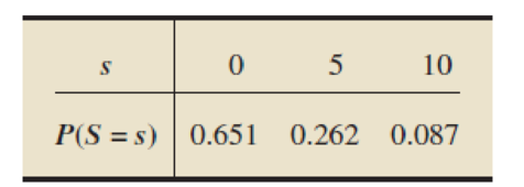
- a. On average, how many points will the archer score per arrow shot?
- b. Obtain and interpret the standard deviation of the score per arrow shot.
Want to see the full answer?
Check out a sample textbook solution
Chapter 5 Solutions
Introductory Statistics (10th Edition)
Additional Math Textbook Solutions
Pathways To Math Literacy (looseleaf)
Elementary Statistics: Picturing the World (7th Edition)
Basic College Mathematics
Finite Mathematics for Business, Economics, Life Sciences and Social Sciences
Introductory Statistics
Mathematics for the Trades: A Guided Approach (11th Edition) (What's New in Trade Math)


- Suppose we wish to test the hypothesis that women with a sister’s history of breast cancer are at higher risk of developing breast cancer themselves. Suppose we assume that the prevalence rate of breast cancer is 3% among 60- to 64-year-old U.S. women, whereas it is 5% among women with a sister history. We propose to interview 400 women 40 to 64 years of age with a sister history of the disease. What is the power of such a study assuming that the level of significance is 10%? I only need help writing the null and alternative hypotheses.arrow_forward4.96 The breaking strengths for 1-foot-square samples of a particular synthetic fabric are approximately normally distributed with a mean of 2,250 pounds per square inch (psi) and a standard deviation of 10.2 psi. Find the probability of selecting a 1-foot-square sample of material at random that on testing would have a breaking strength in excess of 2,265 psi.4.97 Refer to Exercise 4.96. Suppose that a new synthetic fabric has been developed that may have a different mean breaking strength. A random sample of 15 1-foot sections is obtained, and each section is tested for breaking strength. If we assume that the population standard deviation for the new fabric is identical to that for the old fabric, describe the sampling distribution forybased on random samples of 15 1-foot sections of new fabricarrow_forwardUne Entreprise œuvrant dans le domaine du multividéo donne l'opportunité à ses programmeurs-analystes d'évaluer la performance des cadres supérieurs. Voici les résultats obtenues (sur une échelle de 10 à 50) où 50 représentent une excellente performance. 10 programmeurs furent sélectionnés au hazard pour évaluer deux cadres. Un rapport Excel est également fourni. Programmeurs Cadre A Cadre B 1 34 36 2 32 34 3 18 19 33 38 19 21 21 23 7 35 34 8 20 20 9 34 34 10 36 34 Test d'égalité des espérances: observations pairéesarrow_forward
- A television news channel samples 25 gas stations from its local area and uses the results to estimate the average gas price for the state. What’s wrong with its margin of error?arrow_forwardYou’re fed up with keeping Fido locked inside, so you conduct a mail survey to find out people’s opinions on the new dog barking ordinance in a certain city. Of the 10,000 people who receive surveys, 1,000 respond, and only 80 are in favor of it. You calculate the margin of error to be 1.2 percent. Explain why this reported margin of error is misleading.arrow_forwardYou find out that the dietary scale you use each day is off by a factor of 2 ounces (over — at least that’s what you say!). The margin of error for your scale was plus or minus 0.5 ounces before you found this out. What’s the margin of error now?arrow_forward
- Suppose that Sue and Bill each make a confidence interval out of the same data set, but Sue wants a confidence level of 80 percent compared to Bill’s 90 percent. How do their margins of error compare?arrow_forwardSuppose that you conduct a study twice, and the second time you use four times as many people as you did the first time. How does the change affect your margin of error? (Assume the other components remain constant.)arrow_forwardOut of a sample of 200 babysitters, 70 percent are girls, and 30 percent are guys. What’s the margin of error for the percentage of female babysitters? Assume 95 percent confidence.What’s the margin of error for the percentage of male babysitters? Assume 95 percent confidence.arrow_forward
- You sample 100 fish in Pond A at the fish hatchery and find that they average 5.5 inches with a standard deviation of 1 inch. Your sample of 100 fish from Pond B has the same mean, but the standard deviation is 2 inches. How do the margins of error compare? (Assume the confidence levels are the same.)arrow_forwardA survey of 1,000 dental patients produces 450 people who floss their teeth adequately. What’s the margin of error for this result? Assume 90 percent confidence.arrow_forwardThe annual aggregate claim amount of an insurer follows a compound Poisson distribution with parameter 1,000. Individual claim amounts follow a Gamma distribution with shape parameter a = 750 and rate parameter λ = 0.25. 1. Generate 20,000 simulated aggregate claim values for the insurer, using a random number generator seed of 955.Display the first five simulated claim values in your answer script using the R function head(). 2. Plot the empirical density function of the simulated aggregate claim values from Question 1, setting the x-axis range from 2,600,000 to 3,300,000 and the y-axis range from 0 to 0.0000045. 3. Suggest a suitable distribution, including its parameters, that approximates the simulated aggregate claim values from Question 1. 4. Generate 20,000 values from your suggested distribution in Question 3 using a random number generator seed of 955. Use the R function head() to display the first five generated values in your answer script. 5. Plot the empirical density…arrow_forward
 Algebra & Trigonometry with Analytic GeometryAlgebraISBN:9781133382119Author:SwokowskiPublisher:Cengage