Concept explainers
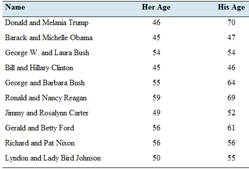
Presidents and first ladies: The presents the ages of the last 10 U.S. presidents and their wives on the first day of their presidencies.

- Compute the least-squares regression line for predicting the president’s age from the first lady’s age.
- Compute the coefficient of determination-
- Construct a
scatterplot of the presidents' ages (y) versus the first ladies' ages (x). - Which point is an outlier?
- Remove die outlier and compute the least-squares regression line for predicting the president’s age from the first lady: s age.
- Is the outlier influential? Explain.
- Compute the coefficient of determination for the data set with the outlier removed. Is due proportion of variation explained by due least-squares regression he greater, less. or about the same without due outlier? Explain.
a.
To Calculate: The least-squares regression line for predicting the president’s age from lady’s age.
Answer to Problem 24E
The least-squares regression line is,
Explanation of Solution
Given: The following table presents the age of the president’s and their wives on the first day of their presidencies.
| Name | Her Age | His Age |
| Donald and Melania Trump | 46 | 70 |
| Barak and Mechelle Obama | 45 | 47 |
| George W. and Laura Bush | 54 | 54 |
| Bill and Hillary Clinton | 45 | 46 |
| George and Babara Bush | 55 | 64 |
| Ronald and Nancy Reagan | 59 | 69 |
| Jimmy and Rosalyn Carter | 49 | 52 |
| Gerald and Betty Ford | 56 | 61 |
| Richard and Pat Nixon | 56 | 56 |
| Lyndon and Lady Bird Johnson | 50 | 55 |
Calculation:
Here,
From below formula we can find least regression line.
where
We can find these constants from below formulas.
Where,
| Descriptive Statistics | |||
| N | Mean | Std. Deviation | |
| His age | 10 | 57.40 | 8.409 |
| Her age | 10 | 51.50 | 5.148 |
| Valid N (listwise) | 10 | ||
To find constants,
And,
By substituting above formula,
Conclusion:
The least-squares regression line for predicting the president’s age from lady’s age is,
b.
To find: The correlation coefficient of the two variables.
Answer to Problem 24E
The correlation coefficient is found to be,
Explanation of Solution
Calculation:
The correlation coefficient
Where
The means and the standard deviations of the both variables can be obtained by using the Excel.
| Descriptive Statistics | |||
| N | Mean | Std. Deviation | |
| His age | 10 | 57.40 | 8.409 |
| Her age | 10 | 51.50 | 5.148 |
| Valid N (listwise) | 10 | ||
Then,
Then, a table should be constructed to calculate
The correlation coefficient can be calculated as,
Conclusion:
The correlation coefficient between the interest rates for two mortgage plans is found tobe,
c.
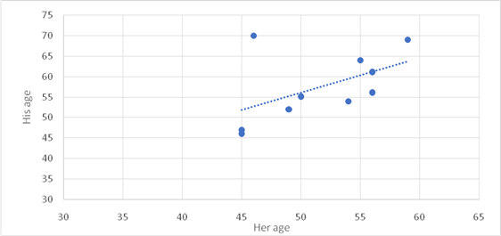
To graph: The scatter plot of the given two quantitative variables.
Explanation of Solution
Graph:
Let

Interpretation:
Out of all these
d.
To Identify: The outliers within the given data.
Answer to Problem 24E
There is one outlier which is age
Explanation of Solution
Explain:
Here, Excel is used to calculate below statistics.
The interquartile range is equal to
To calculate upper bound,
To calculate lower bound,
An outlier is a data point that lies outside the upper bound and lower bound.
Out of all
e.
To find: The least-squares regression line for predicting the president’s age from lady’s age with removing outlier.
Answer to Problem 24E
The least-squares regression is,
Explanation of Solution
Calculation:
Here,
From below formula we can find least regression line.
where
We can find constants from below formulas.
Where,
When the outlier is removed, the number of ordered pairs is
| Descriptive Statistics | |||
| N | Mean | Std. Deviation | |
| His age | 9 | 56.00 | 7.583 |
| Her age | 9 | 52.11 | 5.061 |
| Valid N (listwise) | 9 | ||
To find constants,
And,
By substituting into the above formula,
Conclusion:
The least-squares regression line for predicting the president’s age from lady’s age is,
f.
To Check: The influence of outlier.
Answer to Problem 24E
Yes. It is influenced.
Explanation of Solution
Explain:
| Descriptive Statistics | |||
| N | Mean | Std. Deviation | |
| His age | 10 | 57.40 | 8.409 |
| Her age | 10 | 51.50 | 5.148 |
| Valid N (listwise) | 10 | ||
| Descriptive Statistics | |||
| N | Mean | Std. Deviation | |
| His age | 9 | 56.00 | 7.583 |
| Her age | 9 | 52.11 | 5.061 |
| Valid N (listwise) | 9 | ||
To calculate above statistics, Excel is used. Here we can see statistics with outlier and without outlier. Second table shows statistics without outlier. Total number of observations, mean and standard deviation of dependent and independent variables are changed. So, it influences to least squares regression line for predicting the president’s age from lady’s age.
g.
To find: The correlation coefficient of the two variables without outlier.
Answer to Problem 24E
The correlation coefficient is found to be,
Explanation of Solution
Calculation:
The correlation coefficient
Where
The means and the standard deviations of the both variables can be obtained by using the Excel.
For the remaining
| Descriptive Statistics | |||
| N | Mean | Std. Deviation | |
| His age | 9 | 56.00 | 7.583 |
| Her age | 9 | 52.11 | 5.061 |
| Valid N (listwise) | 9 | ||
Then,
Then, a table should be constructed to calculate
The correlation coefficient can be calculated as,
Conclusion:
The correlation coefficient between the interest rates for two mortgage plans is found to be,
Want to see more full solutions like this?
Chapter 4 Solutions
Connect Hosted by ALEKS Online Access for Elementary Statistics
- The following data show the year to date percent change (YTD % Change) for 30 stock-market indexes from around the word (The Wall Street Journal, August 26, 2013). Click on the datafile logo to reference the data. DATA file Country Australia Index S&P/ASX200 YTD % Change 10.2 Belgium Bel-20 12.6 Brazil São Paulo Bovespa -14.4 Canada S&P/TSX Comp 2.6 Chile Santiago IPSA -16.3 China Shanghai Composite -9.3 Eurozone EURO Stoxx 10.0 France CAC 40 11.8 Germany DAX 10.6 Hong Kong Hang Seng -3.5 India S&P BSE Sensex -4.7 Israel Tel Aviv 1.3 Italy FTSE MIB 6.6 Japan Nikkei 31.4 Mexico IPC All-Share -6.4 Netherlands AEX 9.3 Singapore Straits Times -2.5 South Korea Kospi -6.4 Spain IBEX 35 6.4 Sweden Switzerland SX All Share 13.8 Swiss Market 17.4 Taiwan Weighted 2.3 U.K. FTSE 100 10.1 U.S. S&P 500 16.6 U.S. DJIA 14.5 U.S. Dow Jones Utility 6.6 U.S. Nasdaq 100 17.4 U.S. Nasdaq Composite 21.1 World DJ Global ex U.S. 4.2 World DJ Global Index 9.9 a. What index has the largest positive YTD %…arrow_forwardDescribe a three step process you choose to determine how many elementary schools there are in the city of 5 million people.arrow_forwardQuiz: Exam 1 (Ch 1-4) z Scores Table-3.pdf x + edu/courses/308627/quizzes/2442507/take/questions/48957332 Canvas Hall It browser 5 Connect Set as default incorrect. • This exam is NOT resumable. Meaning, once you start the exam, you must complete it in its entirety. Any blank questions will be marked as By taking this exam, you agree to adhere to the academic integrity standards, which consist of NOT cheating in any way. To get the highest possible score, you are encouraged to review your notes before taking the exam. You may use your notes during the exam, but note that you should be familiar with the concepts and formulas before taking exam. z Scores Table.pdf Question 3 3 pts Here is a data from a survey asking young children how many hours they spend playing video games. The researchers reported the percent of boys and girls who played no games, less than 1 hour per day, 1-3 hours per day, or greater than 3 hours per day. The most common number of hours per day that boys played is…arrow_forward
- Write a Regression summary explaining significance of mode, explaining regression coefficients, significance of the independent variables, R and R square. Premiums earned Net income Dividends Underwriting Gain/ Loss 30.2 1.6 0.6 0.1 47.2 0.6 0.7 -3.6 92.8 8.4 1.8 -1.5 95.4 7.6 2 -4 100.4 6.3 2.2 -8.1 104.9 6.3 2.4 -10.8 113.2 2.2 2.3 -18.2 130.3 3.0 2.4 -21.4 161.9 13.5 2.3 -12.8 182.5 14.9 2.9 -5.9 193.3 11.7 2.9 -7.6arrow_forward1- Let A = {A1, A2, ...), in which A, A, = 0, when i j. a) Is A a π-system? If not, which element(s) should be added to A to become a π-system? b) Prove that σ(A) consists of the finite or countable unions of elements of A; i.c., A E σ(A) if and only if there exists finite or countable sequence {n} such that A = U₁An (Hint: Let F be such class; prove that F is a σ-filed containing A.) c) Let p ≥ 0 be a sequence of non-negative real numbers with Σip₁ = 1. Using p₁'s, how do you construct a probability measure on σ(A)? (Hint: use extension theorem.) 2- Construct an example for which P(lim sup A,) = 1 and P(lim inf An) = 0.arrow_forwardIn a town with 5000 adults, a sample of 50 is selected using SRSWOR and asked their opinion of a proposed municipal project; 30 are found to favor it and 20 oppose it. If, in fact, the adults of the town were equally divided on the proposal, what would be the probability of observing what has been observed? Approximate using the Binomial distribution. Compare this with the exact probability which is 0.0418.arrow_forward
- Good explanation it sure experts solve itarrow_forwardBest explains it not need guidelines okkarrow_forwardActiv Determine compass error using amplitude (Sun). Minimum number of times that activity should be performed: 3 (1 each phase) Sample calculation (Amplitude- Sun): On 07th May 2006 at Sunset, a vessel in position 10°00'N 010°00'W observed the Sun bearing 288° by compass. Find the compass error. LMT Sunset: LIT: (+) 00d 07d 18h 00h 13m 40m UTC Sunset: 07d 18h 53m (added- since longitude is westerly) Declination (07d 18h): N 016° 55.5' d (0.7): (+) 00.6' Declination Sun: N 016° 56.1' Sin Amplitude = Sin Declination/Cos Latitude = Sin 016°56.1'/ Cos 10°00' = 0.295780189 Amplitude=W17.2N (The prefix of amplitude is named easterly if body is rising, and westerly if body is setting. The suffix is named same as declination) True Bearing=287.2° Compass Bearing= 288.0° Compass Error = 0.8° Westarrow_forward
- Only sure experts solve it correct complete solutions okkarrow_forward13. In 2000, two organizations conducted surveys to ascertain the public's opinion on banning gay men from serving in leadership roles in the Boy Scouts.• A Pew poll asked respondents whether they agreed with "the recent decision by the Supreme Court" that "the Boy Scouts of America have a constitutional right to block gay men from becoming troop leaders."A Los Angeles Times poll asked respondents whether they agreed with the following statement: "A Boy Scout leader should be removed from his duties as a troop leader if he is found out to be gay, even if he is considered by the Scout organization to be a model Boy Scout leader."One of these polls found 36% agreement; the other found 56% agreement. Which of the following statements is true?A) The Pew poll found 36% agreement, and the Los Angeles Times poll found 56% agreement.B) The Pew poll includes a leading question, while the Los Angeles Times poll uses neutral wording.C) The Los Angeles Times Poll includes a leading question, while…arrow_forwardAnswer questions 2arrow_forward
 Glencoe Algebra 1, Student Edition, 9780079039897...AlgebraISBN:9780079039897Author:CarterPublisher:McGraw Hill
 Big Ideas Math A Bridge To Success Algebra 1: Stu...AlgebraISBN:9781680331141Author:HOUGHTON MIFFLIN HARCOURTPublisher:Houghton Mifflin Harcourt
 Holt Mcdougal Larson Pre-algebra: Student Edition...AlgebraISBN:9780547587776Author:HOLT MCDOUGALPublisher:HOLT MCDOUGAL
 Linear Algebra: A Modern IntroductionAlgebraISBN:9781285463247Author:David PoolePublisher:Cengage Learning
 Elementary Linear Algebra (MindTap Course List)AlgebraISBN:9781305658004Author:Ron LarsonPublisher:Cengage Learning


