
Concept explainers
Hot enough for you? The following table presents the temperature, in degrees Fahrenheit, and barometric pressure, in inches of mercury, on August 15 at 12 noon in Macon. Georgia; over a nine-year period.
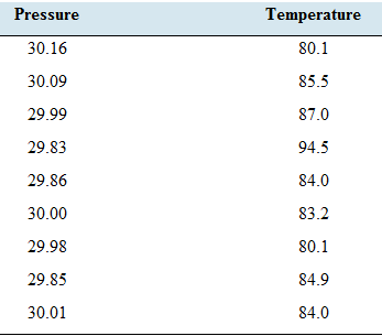
- Compute the least-squares regression line for predicting temperature from barometric pressure.
- Compute file coefficient of determination.
- Construct a
scatterplot of due temperature (y) versus the barometric pressure (x). - Which point is an outlier?
- Remove outlier and compute least-squares regression line for predicting temperature from barometric pressure.
- Is the outlier Explain.
- Compute the coefficient of determination for the data set with the outlier removed. Is the proportion of variation explained by the least-squares regression fine greater, less, or about the same without die outlier? Explain.
a.
The least squares regression line for the given data set.
Answer to Problem 23E
Explanation of Solution
Given information:
Belowtable represents the temperature, in degrees Fahrenheit, and barometric pressure, in inches of mercury, on August

Formula used:
The equation for least-square regression line:
Where
The correlation coefficient of a data is given by:
Where,
The standard deviations are given by:
Calculation:
The mean of x is given by:
The mean of y is given by:
The data can be represented in tabular form as:
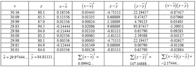
Hence, the standard deviation is given by:
And,
Consider,
Putting the values in the formula,
Putting the values to obtain
Putting the values to obtain
Hence, the least-square regression line is given by:
Therefore, the least squares regression line for the given data set is
b.
The coefficient of determination.
Answer to Problem 23E
Explanation of Solution
Given information:
Same as part
Calculation:
From part
The coefficient of determination is given by:
Where
Putting the values to obtain Coefficient of Determination,
Therefore, the Coefficient of Determination is
c.
Construct the scatterplot of the temperature
Explanation of Solution
Given information:
Below table represents the temperature, in degrees Fahrenheit, and barometric pressure, in inches of mercury, on August

Calculation:
The scatter plot can be drawn with the help of the given data. The Pressure will be taken on horizontal axis and the temperature will betaken on vertical axis.
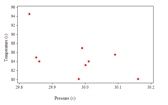
From the scatterplot, it is observed that there is a moderate association between the “variable temperature” and “barometric pressure”.
d.
The points which are outliers.
Answer to Problem 23E
Explanation of Solution
Given information:
Same as part
Calculation:
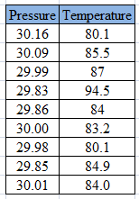
From above table, it can be seen that among all the
Therefore, the outlier point is
e.
The least squares regression line for the given data set excluding the outlier.
Answer to Problem 23E
Explanation of Solution
Given information:
Same as part
Formula used:
The equation for least-square regression line:
Where
The correlation coefficient of a data is given by:
Where,
The standard deviations are given by:
Calculation:
From part
Excluding the outlier,
The mean of
The mean of
The data can be represented in tabular form as:
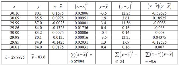
Hence, the standard deviation is given by:
And,
Consider,
Putting the values in the formula,
Putting the values to obtain
Plugging the values to obtain
Hence, the least-square regression line is given by:
Therefore, the least squares regression line for the given data set by excluding the outlier is
f.
Whether the outlier is influential.
Answer to Problem 23E
The outlier is influential.
Explanation of Solution
Given information:
Same as part
Calculation:
From part
From part
From above equations, it can be observed that removing the outlier creates a great difference in the equation of the least square regression line.
Therefore, the outlier is influential.
g.
The coefficient of determination for the data set excluding the outliers.
Answer to Problem 23E
The proportion of variation is less without the outlier.
Explanation of Solution
Given information:
Same as part
Calculation:
The coefficient of determination is given by:
Where
From part
Putting the values to obtain Coefficient of Determination,
Therefore, the Coefficient of Determination is
Here the coefficient of determination reduced without the outlier.
Hence, the proportion of variance explained is less without the outlier.
Want to see more full solutions like this?
Chapter 4 Solutions
Connect Hosted by ALEKS Online Access for Elementary Statistics
- In a town with 5000 adults, a sample of 50 is selected using SRSWOR and asked their opinion of a proposed municipal project; 30 are found to favor it and 20 oppose it. If, in fact, the adults of the town were equally divided on the proposal, what would be the probability of observing what has been observed? Approximate using the Binomial distribution. Compare this with the exact probability which is 0.0418.arrow_forwardGood explanation it sure experts solve itarrow_forwardBest explains it not need guidelines okkarrow_forward
- Activ Determine compass error using amplitude (Sun). Minimum number of times that activity should be performed: 3 (1 each phase) Sample calculation (Amplitude- Sun): On 07th May 2006 at Sunset, a vessel in position 10°00'N 010°00'W observed the Sun bearing 288° by compass. Find the compass error. LMT Sunset: LIT: (+) 00d 07d 18h 00h 13m 40m UTC Sunset: 07d 18h 53m (added- since longitude is westerly) Declination (07d 18h): N 016° 55.5' d (0.7): (+) 00.6' Declination Sun: N 016° 56.1' Sin Amplitude = Sin Declination/Cos Latitude = Sin 016°56.1'/ Cos 10°00' = 0.295780189 Amplitude=W17.2N (The prefix of amplitude is named easterly if body is rising, and westerly if body is setting. The suffix is named same as declination) True Bearing=287.2° Compass Bearing= 288.0° Compass Error = 0.8° Westarrow_forwardOnly sure experts solve it correct complete solutions okkarrow_forward13. In 2000, two organizations conducted surveys to ascertain the public's opinion on banning gay men from serving in leadership roles in the Boy Scouts.• A Pew poll asked respondents whether they agreed with "the recent decision by the Supreme Court" that "the Boy Scouts of America have a constitutional right to block gay men from becoming troop leaders."A Los Angeles Times poll asked respondents whether they agreed with the following statement: "A Boy Scout leader should be removed from his duties as a troop leader if he is found out to be gay, even if he is considered by the Scout organization to be a model Boy Scout leader."One of these polls found 36% agreement; the other found 56% agreement. Which of the following statements is true?A) The Pew poll found 36% agreement, and the Los Angeles Times poll found 56% agreement.B) The Pew poll includes a leading question, while the Los Angeles Times poll uses neutral wording.C) The Los Angeles Times Poll includes a leading question, while…arrow_forward
- Introduce yourself and describe a time when you used data in a personal or professional decision. This could be anything from analyzing sales data on the job to making an informed purchasing decision about a home or car. Describe to Susan how to take a sample of the student population that would not represent the population well. Describe to Susan how to take a sample of the student population that would represent the population well. Finally, describe the relationship of a sample to a population and classify your two samples as random, systematic, cluster, stratified, or convenience.arrow_forward1.2.17. (!) Let G,, be the graph whose vertices are the permutations of (1,..., n}, with two permutations a₁, ..., a,, and b₁, ..., b, adjacent if they differ by interchanging a pair of adjacent entries (G3 shown below). Prove that G,, is connected. 132 123 213 312 321 231arrow_forwardYou are planning an experiment to determine the effect of the brand of gasoline and the weight of a car on gas mileage measured in miles per gallon. You will use a single test car, adding weights so that its total weight is 3000, 3500, or 4000 pounds. The car will drive on a test track at each weight using each of Amoco, Marathon, and Speedway gasoline. Which is the best way to organize the study? Start with 3000 pounds and Amoco and run the car on the test track. Then do 3500 and 4000 pounds. Change to Marathon and go through the three weights in order. Then change to Speedway and do the three weights in order once more. Start with 3000 pounds and Amoco and run the car on the test track. Then change to Marathon and then to Speedway without changing the weight. Then add weights to get 3500 pounds and go through the three gasolines in the same order.Then change to 4000 pounds and do the three gasolines in order again. Choose a gasoline at random, and run the car with this gasoline at…arrow_forward
 Glencoe Algebra 1, Student Edition, 9780079039897...AlgebraISBN:9780079039897Author:CarterPublisher:McGraw Hill
 Big Ideas Math A Bridge To Success Algebra 1: Stu...AlgebraISBN:9781680331141Author:HOUGHTON MIFFLIN HARCOURTPublisher:Houghton Mifflin Harcourt
 Functions and Change: A Modeling Approach to Coll...AlgebraISBN:9781337111348Author:Bruce Crauder, Benny Evans, Alan NoellPublisher:Cengage Learning
 Trigonometry (MindTap Course List)TrigonometryISBN:9781337278461Author:Ron LarsonPublisher:Cengage LearningAlgebra & Trigonometry with Analytic GeometryAlgebraISBN:9781133382119Author:SwokowskiPublisher:Cengage


