Concept explainers
Videos
a.
Arrange the data and obtain Xmin and Xmax.
a.
Answer to Problem 99CE
The value of Xmin is 0.9.
The value of Xmax is 11.9.
Explanation of Solution
Calculation:
The data state to choose a dataset to prepare a brief descriptive report.
Here, the data chosen is Data set A.
The Data set A represents the percentage of sales in selected industries.
The data set A of sales percent can be sorted either ascending or descending.
Here, the data is sorted in the ascending order.
Sorting:
Software procedure:
Step-by-step procedure to sort the data using the MINITAB software is given below:
- Choose Data > Sort.
- In columns to sort by, enter Percent.
- Under Columns to sort , Choose specified columns.
- In columns, enter the percent and choose increasing option.
- In storage location for current columns, choose “specified columns of the current worksheet”.
- In columns, enter “sorted percent”.
- Click ok.
Thus, the sorted data has been stored in the column of sorted percent.
Minimum and Maximum:
Step-by-step procedure to find the minimum and maximum using the MINITAB software using the given below:
- Choose Calc>calculator.
- In store result in variable box, enter Minimum.
- Under Expression, enter “MIN(Percent)”.
- Click ok.
- Choose Calc>calculator.
- In store result in variable box, enter Maximum.
- Under Expression, enter “MAX(Percent)”.
- Click ok.
Data display:
Step-by-step procedure to display the data using the MINITAB software using the given below:
- Choose data> display data.
- Select the columns to display as Minimum, Maximum.
- Click ok.
Output using the MINITAB software is given below:
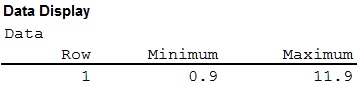
Thus, the value of Xmin is 0.9 and the value of Xmax is 11.9.
b.
Construct a histogram.
b.
Answer to Problem 99CE
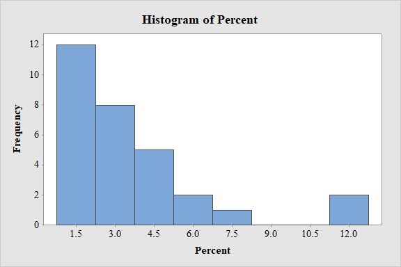
Histogram:
Output obtained from MINITAB software is:
Explanation of Solution
Calculation:
Software procedure:
- Step by step procedure to draw the Histogram using MINITAB software is given below:
- Choose Graph > Histogram.
- Choose Simple, and then click OK.
- In Graph variables, enter the Percent.
- Click OK.
Thus, the histogram has been obtained.
By observing the graph, it is clear that the curve is right skewed. Hence, it is appropriate to conclude that the data is approximately right skewed. Thus, the data set A for percent of sales is approximately right skewed.
c.
Find the
c.
Answer to Problem 99CE
The mean score is 3.55.
The median score is 3.
Explanation of Solution
Mean and median:
Software procedure:
Step-by-step procedure to find the mean, the median using the MINITAB software is given below:
- Choose Stat > Basic Statistics > Display
Descriptive Statistics . - In Variables enter the columns Percent.
- Choose option statistics, and select Mean, Median.
- Click OK.
Output using the MINITAB software is given below:
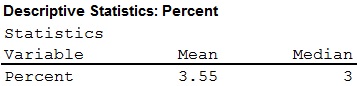
- Thus, the mean and the median for the data set A are 3.55 and 3 respectively.
Shape of the distribution:
- For symmetric data, the mean, the median and the
mode are equal. - For positively skewed data, the mean exceeds the median.
- For negatively skewed data, the mean is lower than the median.
From the value of mean, median, it is observed that the value of mean is greater than that of the median.
Thus, the data is said to be right skewed or positively skewed.
d.
Find the standard deviation for data set A.
d.
Answer to Problem 99CE
The standard deviation for data set A is 2.749.
Explanation of Solution
Standard deviation:
Software procedure:
Step-by-step procedure to find the mean and standard deviation using the MINITAB software is given below:
- Choose Stat > Basic Statistics > Display Descriptive Statistics.
- In Variables enter the columns Percent.
- Choose option statistics, and select Standard deviation.
- Click OK.
Output using the MINITAB software is given below:
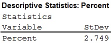
- Thus, the standard deviation have been obtained.
e.
Standardize the data and identify the outliers and unusual observations.
e.
Answer to Problem 99CE
The standardized values of dataset A are given below:
| -0.9640 | -0.6366 | 0.3456 | 0.3820 | -0.6730 | 0.0909 |
| 0.7093 | -0.0182 | -0.0182 | -0.9276 | -0.1637 | -0.2001 |
| 1.4005 | -0.9640 | -0.8912 | -0.0182 | 3.0375 | -0.6002 |
| -0.8185 | 1.0367 | -0.2001 | -0.4547 | 0.2728 | -0.6366 |
| -0.8912 | -0.5638 | -0.5638 | 0.4911 | -0.3820 | 2.8192 |
There are one outlier in the dataset.
Explanation of Solution
Standardized values:
Software procedure:
Step-by-step software procedure to obtain standardized values using EXCEL software is as follows:
- Open an EXCEL file.
- Enter the data in the column A in cells A1 to A32.
- In cell B1, enter the formula “=STANDARDIZE(A1, 3.55, 2.749)”.
- Select “ENTER” option.
- Select and copy the cell B1 and drag till the 30nd cell.
- Output using EXCEL software is given below:
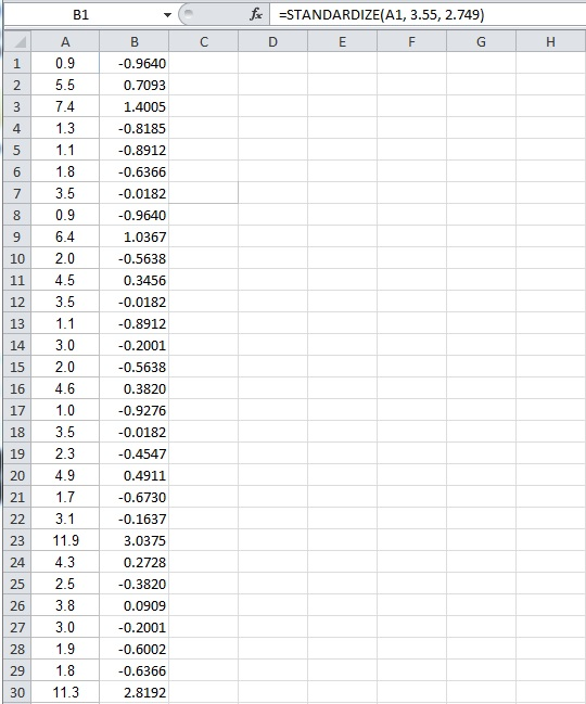
Thus, the standardized values have been obtained using EXCEL.
The outliers in the data set A can be identified using
Empirical Rule:
The Empirical Rule for a Normal model states that:
- Within 1 standard deviation of mean, 68.26% of all observations will lie.
- Within 2 standard deviations of mean, 95.44% of all observations will lie.
- Within 3 standard deviations of mean, 99.73% of all observations will lie.
Empirical rule using MEGASTAT:
Software procedure:
Step-by-step software procedure to obtain Empirical rule using Mega Stat software is as follows:
- Open an EXCEL file.
- Enter the data in the column A in cells A1 to A30.
- From the Add-Ins, Select Mega Stat >Descriptive statistics.
- A dialogue box appears.
- In Input
range box, select the input range from Sheet1!$A$1:$A$30. - From the list box, select Empirical rule.
- Click “OK”.
Output obtained using MEGA STAT is as follows:
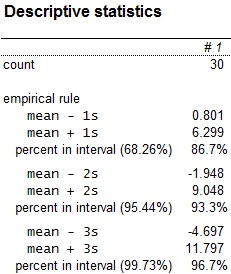
The upper and lower bounds for the intervals indicated by the Empirical rule have been obtained.
Based on the z-scores, the observation has one outlier, that is, the observations with values 11.9 do not lie within the 3-standard deviations limits (–4.697 to 11.797). there is no unusual observation in the data set A.
f.
Find the
f.
Answer to Problem 99CE
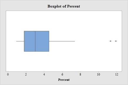
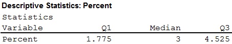
The Q1 (25th percentile) is 1.775, Q2 (50th percentile) is 3 and Q3 (75th percentile) is 4.525.
The boxplot for the data set A is:
Explanation of Solution
Quartiles:
Software procedure:
Step-by-step procedure to find the Quartiles using the MINITAB software:
- Choose Stat > Basic Statistics > Display Descriptive Statistics.
- In Variables enter the columns Percent.
- Choose option statistics, and select First Quartile, Median and Third Quartile.
- Choose option Graphs, and select boxplot of data.
- Click OK.
Output using the MINITAB software is given below:
- Thus, the Quartiles and boxplot have been obtained.
Observation:
From the boxplot, it is observed that the data set has two outliers within it. The boxplot disclosed that the median is closer to the first quartile, Q1 than it is to the third quartile, Q3, suggesting that the data is right skewed. The whiskers on the two sides are close in length, although it appears that the left whisker is slightly longer.
Want to see more full solutions like this?
Chapter 4 Solutions
APPLIED STAT.IN BUS.+ECONOMICS


- 1. [20] The joint PDF of RVs X and Y is given by xe-(z+y), r>0, y > 0, fx,y(x, y) = 0, otherwise. (a) Find P(0X≤1, 1arrow_forward4. [20] Let {X1,..., X} be a random sample from a continuous distribution with PDF f(x; 0) = { Axe 5 0, x > 0, otherwise. where > 0 is an unknown parameter. Let {x1,...,xn} be an observed sample. (a) Find the value of c in the PDF. (b) Find the likelihood function of 0. (c) Find the MLE, Ô, of 0. (d) Find the bias and MSE of 0.arrow_forward3. [20] Let {X1,..., Xn} be a random sample from a binomial distribution Bin(30, p), where p (0, 1) is unknown. Let {x1,...,xn} be an observed sample. (a) Find the likelihood function of p. (b) Find the MLE, p, of p. (c) Find the bias and MSE of p.arrow_forwardGiven the sample space: ΩΞ = {a,b,c,d,e,f} and events: {a,b,e,f} A = {a, b, c, d}, B = {c, d, e, f}, and C = {a, b, e, f} For parts a-c: determine the outcomes in each of the provided sets. Use proper set notation. a. (ACB) C (AN (BUC) C) U (AN (BUC)) AC UBC UCC b. C. d. If the outcomes in 2 are equally likely, calculate P(AN BNC).arrow_forwardSuppose a sample of O-rings was obtained and the wall thickness (in inches) of each was recorded. Use a normal probability plot to assess whether the sample data could have come from a population that is normally distributed. Click here to view the table of critical values for normal probability plots. Click here to view page 1 of the standard normal distribution table. Click here to view page 2 of the standard normal distribution table. 0.191 0.186 0.201 0.2005 0.203 0.210 0.234 0.248 0.260 0.273 0.281 0.290 0.305 0.310 0.308 0.311 Using the correlation coefficient of the normal probability plot, is it reasonable to conclude that the population is normally distributed? Select the correct choice below and fill in the answer boxes within your choice. (Round to three decimal places as needed.) ○ A. Yes. The correlation between the expected z-scores and the observed data, , exceeds the critical value, . Therefore, it is reasonable to conclude that the data come from a normal population. ○…arrow_forwardding question ypothesis at a=0.01 and at a = 37. Consider the following hypotheses: 20 Ho: μ=12 HA: μ12 Find the p-value for this hypothesis test based on the following sample information. a. x=11; s= 3.2; n = 36 b. x = 13; s=3.2; n = 36 C. c. d. x = 11; s= 2.8; n=36 x = 11; s= 2.8; n = 49arrow_forward13. A pharmaceutical company has developed a new drug for depression. There is a concern, however, that the drug also raises the blood pressure of its users. A researcher wants to conduct a test to validate this claim. Would the manager of the pharmaceutical company be more concerned about a Type I error or a Type II error? Explain.arrow_forwardFind the z score that corresponds to the given area 30% below z.arrow_forwardFind the following probability P(z<-.24)arrow_forward3. Explain why the following statements are not correct. a. "With my methodological approach, I can reduce the Type I error with the given sample information without changing the Type II error." b. "I have already decided how much of the Type I error I am going to allow. A bigger sample will not change either the Type I or Type II error." C. "I can reduce the Type II error by making it difficult to reject the null hypothesis." d. "By making it easy to reject the null hypothesis, I am reducing the Type I error."arrow_forwardGiven the following sample data values: 7, 12, 15, 9, 15, 13, 12, 10, 18,12 Find the following: a) Σ x= b) x² = c) x = n d) Median = e) Midrange x = (Enter a whole number) (Enter a whole number) (use one decimal place accuracy) (use one decimal place accuracy) (use one decimal place accuracy) f) the range= g) the variance, s² (Enter a whole number) f) Standard Deviation, s = (use one decimal place accuracy) Use the formula s² ·Σx² -(x)² n(n-1) nΣ x²-(x)² 2 Use the formula s = n(n-1) (use one decimal place accuracy)arrow_forwardTable of hours of television watched per week: 11 15 24 34 36 22 20 30 12 32 24 36 42 36 42 26 37 39 48 35 26 29 27 81276 40 54 47 KARKE 31 35 42 75 35 46 36 42 65 28 54 65 28 23 28 23669 34 43 35 36 16 19 19 28212 Using the data above, construct a frequency table according the following classes: Number of Hours Frequency Relative Frequency 10-19 20-29 |30-39 40-49 50-59 60-69 70-79 80-89 From the frequency table above, find a) the lower class limits b) the upper class limits c) the class width d) the class boundaries Statistics 300 Frequency Tables and Pictures of Data, page 2 Using your frequency table, construct a frequency and a relative frequency histogram labeling both axes.arrow_forwardarrow_back_iosSEE MORE QUESTIONSarrow_forward_ios
 Glencoe Algebra 1, Student Edition, 9780079039897...AlgebraISBN:9780079039897Author:CarterPublisher:McGraw Hill
 Holt Mcdougal Larson Pre-algebra: Student Edition...AlgebraISBN:9780547587776Author:HOLT MCDOUGALPublisher:HOLT MCDOUGAL
 Big Ideas Math A Bridge To Success Algebra 1: Stu...AlgebraISBN:9781680331141Author:HOUGHTON MIFFLIN HARCOURTPublisher:Houghton Mifflin Harcourt
 College Algebra (MindTap Course List)AlgebraISBN:9781305652231Author:R. David Gustafson, Jeff HughesPublisher:Cengage Learning
 Functions and Change: A Modeling Approach to Coll...AlgebraISBN:9781337111348Author:Bruce Crauder, Benny Evans, Alan NoellPublisher:Cengage Learning