Chapter 3.2, Problem 66E

(a)

To determine

To make: a scatterplot with HbA

Answer to Problem 66E

  

Explanation of Solution

Given:

subject	HbA	FPG	subject	HbA	FPG
1	6.1	141	10	8.7	172
2	6.3	158	11	9.4	200
3	6.4	112	12	10.4	271
4	6.8	153	13	10.6	103
5	7.0	134	14	10.7	172
6	7.1	95	15	10.7	359
7	7.5	96	16	11.2	145
8	7.7	78	17	13.7	147
9	7.9	148	18	19.3	255

Calculation:

Put HbA (the explanatory variable) on the horizontal axis and FPG (the response variable) on the vertical axis.

Using the MINITAB, the scatterplot for the given data is shown below:

  

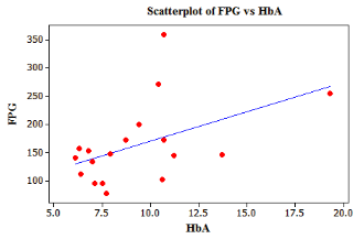
The graph shows a clear direction: the overall pattern moves from lower left to upper right. That is, higher HbA tend to have higher FPG. We call this a positive association between the two variables. The form of the relationship is linear. That is, the overall pattern follows a straight line from lower left to upper right. The relationship is weak because the points deviate greatly from line and there are some outliers.

Conclusion:

Therefore, the required scatterplot is drawn.

(b)

To determine

To find: the correlation for all 18 subjects, for all except subject 15 and for all except subject 18

Answer to Problem 66E

The correlation r with all 18 subjects is r = 0.482

The correlation r without subject 15 is r =0.568

The correlation r without subject 18 is r =0.384

Explanation of Solution

Calculation:

Using the MINITAB, the correlation r with all 18 subjects is r = 0.482

The correlation r without subject 15 is r =0.568

The correlation r without subject 18 is r =0.384

The correlation without subject 15 and without subject 18 is r = 0.324

When we remove outlier subject 15, Correlation increases by 0.086. However, removing subject

15 has little effect on the correlation. Because of subject 15's extreme position on HbA scale; this point has a strong influence on the position of the regression line. When we remove outlier subject 18, Correlation decreases by 0.098. Just one outlier can be entirely responsible for a high value of the correlation that otherwise (without the outlier) would be very low. Needless to say, one should never base important conclusions on the value of the correlation coefficient alone (i.e., examining the respective scatterplot is always recommended). These might be called 'good' outliers.

Both subject 15 and 18 are influential, because the linear correlation coefficient changes significantly, when the subject is removed from the data set.

Conclusion:

Therefore,

The correlation r with all 18 subjects is r = 0.482

The correlation r without subject 15 is r =0.568

The correlation r without subject 18 is r =0.384

(c)

To determine

To explain: whether subject 15 or subject 18 are strongly influential for the least-squares line

Answer to Problem 66E

Subject 15 and subject 18 both are influential.

Explanation of Solution

Calculation:

The below figure shows the least-square lines with all 18 subjects, without subject 15 and without subject 18.

  

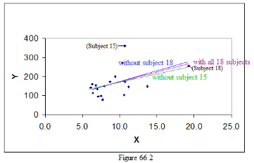
Here it is seen that subject 18 has great importance. This is the point which we can say a good outlier because this point stretches the pattern to upper right direction. If we remove this point correlation drops because rest of the points does not show any clear pattern. Subject 15 has a very large residual because this point lies far from the regression line. Least-squares lines make the sum of squares of the vertical distances to the points as small as possible. A point that is extreme in the X direction with no other points near it pulls the line toward itself. It is called points influential. It reduces the slope of the line.

Conclusion:

Therefore, subject 15 and subject 18 both are influential.