Concept explainers
Videos
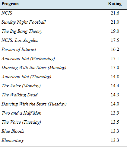
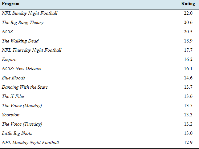
What’s your favorite TV show? The following tables present the numbers of viewers, in millions for the top 15 prime-time shows for the 2012—2013 and 2015—2016 seasons. The numbers of viewers include those who watched the program on any platform, including time-shifting up to seven days after the original telecast.

- Find the population standard deviation of the ratings for 20 12—2013.
- Find the population standard deviation of the ratings for 2015—2016.
- Compute the
range for the ratings for both seasons. - Based on the standard deviations, did the spread in ratings increase or decrease over the two seasons?
- Based on the ranges, did the spread in ratings increase or decrease over the two seasons?
a)
To find: the sample standard deviation of rating 2012 − 2013.
Answer to Problem 39E
Standard deviation = 2.74
Explanation of Solution
Given:
| Top Rated TV Programs: 2012−2013 | Top Rated TV Programs: 2015−2016 | ||
| Program | Rating | Program | Rating |
| NCIS | 21.6 | NFL Sunday Night Football | 22 |
| Sunday Night Football | 21 | The Big Bang Theory | 20.6 |
| The Big Bang Theory | 19 | NCIS | 20.5 |
| NCIS: Los Angeles | 17.5 | The Walking Dead | 18.9 |
| Person of Interest | 16.2 | NFL Thursday Night Football | 17.7 |
| American Idol (Wednesday) | 15.1 | Empire | 16.2 |
| Dancing with the Stars (Monday) | 15 | NCIS: New Orleans | 16.1 |
| American Idol (Thursday) | 14.8 | Blue Bloods | 14.6 |
| The Voice (Monday) | 14.4 | Dancing with the Stars | 13.7 |
| The Walking Dead | 14.3 | The X-Files | 13.6 |
| Dancing with the Stars (Tuesday) | 14 | The Voice (Monday) | 13.5 |
| Two and a Half Men | 13.9 | Scorpion | 13.3 |
| The Voice (Tuesday) | 13.5 | The Voice (Tuesday) | 13.2 |
| Blue Bloods | 13.3 | Little Big Shots | 13 |
| Elementary | 13.3 | NFL Monday Night Football | 12.9 |
Formula used:
Standard Deviation = √∑(xi−ˉx)2n−1
Calculation:
| Top Rated TV Programs: 2012−2013 | ||
| Program | Rating | (xi−ˉx)2 |
| NCIS | 21.6 | 33.72 |
| Sunday Night Football | 21 | 27.11 |
| The Big Bang Theory | 19 | 10.28 |
| NCIS: Los Angeles | 17.5 | 2.91 |
| Person of Interest | 16.2 | 0.17 |
| American Idol (Wednesday) | 15.1 | 0.48 |
| Dancing with the Stars (Monday) | 15 | 0.63 |
| American Idol (Thursday) | 14.8 | 0.99 |
| The Voice (Monday) | 14.4 | 1.94 |
| The Walking Dead | 14.3 | 2.23 |
| Dancing with the Stars (Tuesday) | 14 | 3.22 |
| Two and a Half Men | 13.9 | 3.58 |
| The Voice (Tuesday) | 13.5 | 5.26 |
| Blue Bloods | 13.3 | 6.22 |
| Elementary | 13.3 | 6.22 |
| Sum | 236.90 | 104.95 |
| average | 15.79 | |
| Standard deviation | 2.74 | |
Standard Deviation = √104.9514=2.74
b)
To find: the sample standard deviation for the rating in year 2015 − 2016.
Answer to Problem 39E
Standard deviation = 3.18
Explanation of Solution
Calculation:
| Top Rated TV Programs: 2015−2016 | ||
| Program | Rating | (yi−ˉy)2 |
| NFL Sunday Night Football | 22 | 36.16 |
| The Big Bang Theory | 20.6 | 21.28 |
| NCIS | 20.5 | 20.37 |
| The Walking Dead | 18.9 | 8.49 |
| NFL Thursday Night Football | 17.7 | 2.94 |
| Empire | 16.2 | 0.05 |
| NCIS: New Orleans | 16.1 | 0.01 |
| Blue Bloods | 14.6 | 1.92 |
| Dancing with the Stars | 13.7 | 5.23 |
| The X-Files | 13.6 | 5.70 |
| The Voice (Monday) | 13.5 | 6.18 |
| Scorpion | 13.3 | 7.22 |
| The Voice (Tuesday) | 13.2 | 7.77 |
| Little Big Shots | 13 | 8.92 |
| NFL Monday Night Football | 12.9 | 9.53 |
| Sum | 239.8 | 141.76 |
| average | 15.99 | |
| Standard deviation | 3.18 | |
Standard Deviation = √141.7614=3.18
c)
To find: the range of ratings for both years.
Answer to Problem 39E
Range:
2012 − 13 = 8.3
2015 − 15 = 9.1
Explanation of Solution
Formula used:
Range = Highest Value − lowest value
Calculation:
Range for 2012–2013=21.6–13.3 =8.3
Range for 2015–2016=22−12.9=9.1
d)
To explain: whether the spread has increase or decrease based on standard deviation of both years.
Answer to Problem 39E
Increased
Explanation of Solution
Since the standard deviation in 2012 − 2013 is 2.74 and in year 2015 − 2016 it is 3.18, which shows that the spread of rating has increased over the given time periods.
e)
To explain: whether the spread has increase or decrease based on standard deviation of both years.
Answer to Problem 39E
Increased
Explanation of Solution
Since the Range in 2012 − 2013 is 8.3 and in year 2015 − 2016 it is 9.1, which shows that the spread of rating has increased over the given time periods.
Want to see more full solutions like this?
Chapter 3 Solutions
Elementary Statistics ( 3rd International Edition ) Isbn:9781260092561


- Calculate the 90% confidence interval for the population mean difference using the data in the attached image. I need to see where I went wrong.arrow_forwardMicrosoft Excel snapshot for random sampling: Also note the formula used for the last column 02 x✓ fx =INDEX(5852:58551, RANK(C2, $C$2:$C$51)) A B 1 No. States 2 1 ALABAMA Rand No. 0.925957526 3 2 ALASKA 0.372999976 4 3 ARIZONA 0.941323044 5 4 ARKANSAS 0.071266381 Random Sample CALIFORNIA NORTH CAROLINA ARKANSAS WASHINGTON G7 Microsoft Excel snapshot for systematic sampling: xfx INDEX(SD52:50551, F7) A B E F G 1 No. States Rand No. Random Sample population 50 2 1 ALABAMA 0.5296685 NEW HAMPSHIRE sample 10 3 2 ALASKA 0.4493186 OKLAHOMA k 5 4 3 ARIZONA 0.707914 KANSAS 5 4 ARKANSAS 0.4831379 NORTH DAKOTA 6 5 CALIFORNIA 0.7277162 INDIANA Random Sample Sample Name 7 6 COLORADO 0.5865002 MISSISSIPPI 8 7:ONNECTICU 0.7640596 ILLINOIS 9 8 DELAWARE 0.5783029 MISSOURI 525 10 15 INDIANA MARYLAND COLORADOarrow_forwardSuppose the Internal Revenue Service reported that the mean tax refund for the year 2022 was $3401. Assume the standard deviation is $82.5 and that the amounts refunded follow a normal probability distribution. Solve the following three parts? (For the answer to question 14, 15, and 16, start with making a bell curve. Identify on the bell curve where is mean, X, and area(s) to be determined. 1.What percent of the refunds are more than $3,500? 2. What percent of the refunds are more than $3500 but less than $3579? 3. What percent of the refunds are more than $3325 but less than $3579?arrow_forward
- A normal distribution has a mean of 50 and a standard deviation of 4. Solve the following three parts? 1. Compute the probability of a value between 44.0 and 55.0. (The question requires finding probability value between 44 and 55. Solve it in 3 steps. In the first step, use the above formula and x = 44, calculate probability value. In the second step repeat the first step with the only difference that x=55. In the third step, subtract the answer of the first part from the answer of the second part.) 2. Compute the probability of a value greater than 55.0. Use the same formula, x=55 and subtract the answer from 1. 3. Compute the probability of a value between 52.0 and 55.0. (The question requires finding probability value between 52 and 55. Solve it in 3 steps. In the first step, use the above formula and x = 52, calculate probability value. In the second step repeat the first step with the only difference that x=55. In the third step, subtract the answer of the first part from the…arrow_forwardIf a uniform distribution is defined over the interval from 6 to 10, then answer the followings: What is the mean of this uniform distribution? Show that the probability of any value between 6 and 10 is equal to 1.0 Find the probability of a value more than 7. Find the probability of a value between 7 and 9. The closing price of Schnur Sporting Goods Inc. common stock is uniformly distributed between $20 and $30 per share. What is the probability that the stock price will be: More than $27? Less than or equal to $24? The April rainfall in Flagstaff, Arizona, follows a uniform distribution between 0.5 and 3.00 inches. What is the mean amount of rainfall for the month? What is the probability of less than an inch of rain for the month? What is the probability of exactly 1.00 inch of rain? What is the probability of more than 1.50 inches of rain for the month? The best way to solve this problem is begin by a step by step creating a chart. Clearly mark the range, identifying the…arrow_forwardClient 1 Weight before diet (pounds) Weight after diet (pounds) 128 120 2 131 123 3 140 141 4 178 170 5 121 118 6 136 136 7 118 121 8 136 127arrow_forward
- Client 1 Weight before diet (pounds) Weight after diet (pounds) 128 120 2 131 123 3 140 141 4 178 170 5 121 118 6 136 136 7 118 121 8 136 127 a) Determine the mean change in patient weight from before to after the diet (after – before). What is the 95% confidence interval of this mean difference?arrow_forwardIn order to find probability, you can use this formula in Microsoft Excel: The best way to understand and solve these problems is by first drawing a bell curve and marking key points such as x, the mean, and the areas of interest. Once marked on the bell curve, figure out what calculations are needed to find the area of interest. =NORM.DIST(x, Mean, Standard Dev., TRUE). When the question mentions “greater than” you may have to subtract your answer from 1. When the question mentions “between (two values)”, you need to do separate calculation for both values and then subtract their results to get the answer. 1. Compute the probability of a value between 44.0 and 55.0. (The question requires finding probability value between 44 and 55. Solve it in 3 steps. In the first step, use the above formula and x = 44, calculate probability value. In the second step repeat the first step with the only difference that x=55. In the third step, subtract the answer of the first part from the…arrow_forwardIf a uniform distribution is defined over the interval from 6 to 10, then answer the followings: What is the mean of this uniform distribution? Show that the probability of any value between 6 and 10 is equal to 1.0 Find the probability of a value more than 7. Find the probability of a value between 7 and 9. The closing price of Schnur Sporting Goods Inc. common stock is uniformly distributed between $20 and $30 per share. What is the probability that the stock price will be: More than $27? Less than or equal to $24? The April rainfall in Flagstaff, Arizona, follows a uniform distribution between 0.5 and 3.00 inches. What is the mean amount of rainfall for the month? What is the probability of less than an inch of rain for the month? What is the probability of exactly 1.00 inch of rain? What is the probability of more than 1.50 inches of rain for the month? The best way to solve this problem is begin by creating a chart. Clearly mark the range, identifying the lower and upper…arrow_forward
- Problem 1: The mean hourly pay of an American Airlines flight attendant is normally distributed with a mean of 40 per hour and a standard deviation of 3.00 per hour. What is the probability that the hourly pay of a randomly selected flight attendant is: Between the mean and $45 per hour? More than $45 per hour? Less than $32 per hour? Problem 2: The mean of a normal probability distribution is 400 pounds. The standard deviation is 10 pounds. What is the area between 415 pounds and the mean of 400 pounds? What is the area between the mean and 395 pounds? What is the probability of randomly selecting a value less than 395 pounds? Problem 3: In New York State, the mean salary for high school teachers in 2022 was 81,410 with a standard deviation of 9,500. Only Alaska’s mean salary was higher. Assume New York’s state salaries follow a normal distribution. What percent of New York State high school teachers earn between 70,000 and 75,000? What percent of New York State high school…arrow_forwardPls help asaparrow_forwardSolve the following LP problem using the Extreme Point Theorem: Subject to: Maximize Z-6+4y 2+y≤8 2x + y ≤10 2,y20 Solve it using the graphical method. Guidelines for preparation for the teacher's questions: Understand the basics of Linear Programming (LP) 1. Know how to formulate an LP model. 2. Be able to identify decision variables, objective functions, and constraints. Be comfortable with graphical solutions 3. Know how to plot feasible regions and find extreme points. 4. Understand how constraints affect the solution space. Understand the Extreme Point Theorem 5. Know why solutions always occur at extreme points. 6. Be able to explain how optimization changes with different constraints. Think about real-world implications 7. Consider how removing or modifying constraints affects the solution. 8. Be prepared to explain why LP problems are used in business, economics, and operations research.arrow_forward
 Big Ideas Math A Bridge To Success Algebra 1: Stu...AlgebraISBN:9781680331141Author:HOUGHTON MIFFLIN HARCOURTPublisher:Houghton Mifflin Harcourt
 Glencoe Algebra 1, Student Edition, 9780079039897...AlgebraISBN:9780079039897Author:CarterPublisher:McGraw Hill
 Holt Mcdougal Larson Pre-algebra: Student Edition...AlgebraISBN:9780547587776Author:HOLT MCDOUGALPublisher:HOLT MCDOUGAL
 College Algebra (MindTap Course List)AlgebraISBN:9781305652231Author:R. David Gustafson, Jeff HughesPublisher:Cengage Learning