
Videos
Physician Office Waiting Times. The average waiting time for a patient at an El Paso physician’s office is just over 29 minutes, well above the national average of 21 minutes. In order to address the issue of long patient wait times, some physician’s offices are using wait tracking systems to notify patients of expected wait times. Patients can adjust their arrival times based on this information and spend less time in waiting rooms. The following data show wait times (minutes) for a sample of patients at offices that do not have an office tracking system and wait times for a sample of patients at offices with an office tracking system.
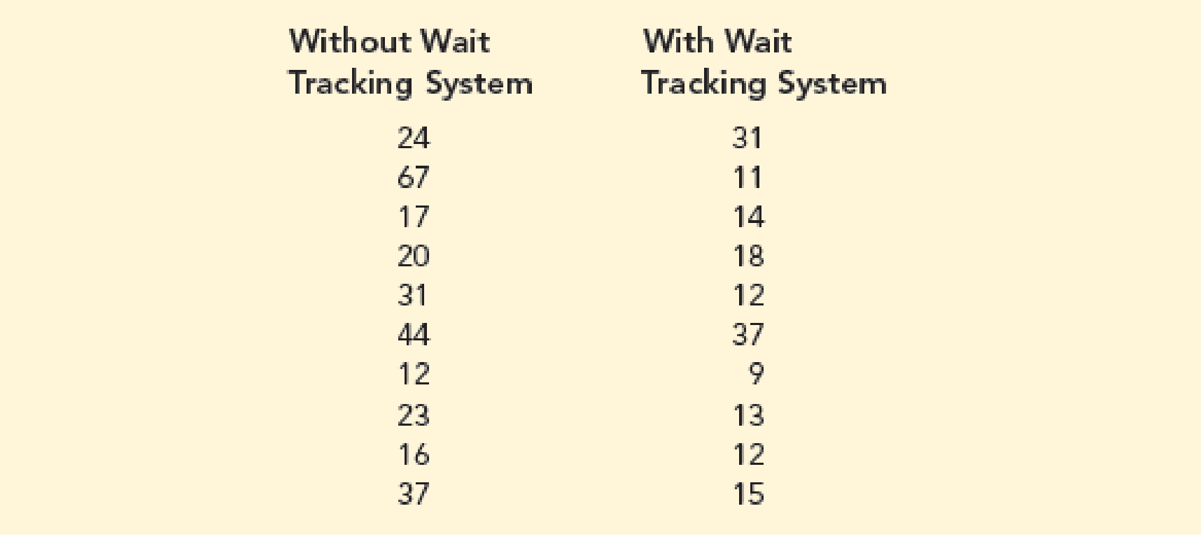
- a. What are the
mean andmedian patient wait times for offices with a wait tracking system? What are the mean and median patient wait times for offices without a wait tracking system? - b. What are the variance and standard deviation of patient wait times for offices with a wait tracking system? What are the variance and standard deviation of patient wait times for visits to offices without a wait tracking system?
- c. Do offices with a wait tracking system have shorter patient wait times than offices without a wait tracking system? Explain.
- d. Considering only offices without a wait tracking system, what is the z-score for the tenth patient in the sample?
- e. Considering only offices with a wait tracking system, what is the z-score for the sixth patient in the sample? How does this z-score compare with the z-score you calculated for part (d)?
- f. Based on z-scores, do the data for offices without a wait tracking system contain any outliers? Based on z-scores, do the data for offices with a wait tracking system contain any outliers?

Trending nowThis is a popular solution!

Chapter 3 Solutions
MindTap Business Statistics, 1 term (6 months) Printed Access Card for Anderson/Sweeney/Williams/Camm/Cochran's Essentials of Statistics for Business and Economics, 8th


- Let X be a random variable with support SX = {−3, 0.5, 3, −2.5, 3.5}. Part ofits probability mass function (PMF) is given bypX(−3) = 0.15, pX(−2.5) = 0.3, pX(3) = 0.2, pX(3.5) = 0.15.(a) Find pX(0.5).(b) Find the cumulative distribution function (CDF), FX(x), of X.1(c) Sketch the graph of FX(x).arrow_forwardA well-known company predominantly makes flat pack furniture for students. Variability with the automated machinery means the wood components are cut with a standard deviation in length of 0.45 mm. After they are cut the components are measured. If their length is more than 1.2 mm from the required length, the components are rejected. a) Calculate the percentage of components that get rejected. b) In a manufacturing run of 1000 units, how many are expected to be rejected? c) The company wishes to install more accurate equipment in order to reduce the rejection rate by one-half, using the same ±1.2mm rejection criterion. Calculate the maximum acceptable standard deviation of the new process.arrow_forward5. Let X and Y be independent random variables and let the superscripts denote symmetrization (recall Sect. 3.6). Show that (X + Y) X+ys.arrow_forward
- 8. Suppose that the moments of the random variable X are constant, that is, suppose that EX" =c for all n ≥ 1, for some constant c. Find the distribution of X.arrow_forward9. The concentration function of a random variable X is defined as Qx(h) = sup P(x ≤ X ≤x+h), h>0. Show that, if X and Y are independent random variables, then Qx+y (h) min{Qx(h). Qr (h)).arrow_forward10. Prove that, if (t)=1+0(12) as asf->> O is a characteristic function, then p = 1.arrow_forward
- 9. The concentration function of a random variable X is defined as Qx(h) sup P(x ≤x≤x+h), h>0. (b) Is it true that Qx(ah) =aQx (h)?arrow_forward3. Let X1, X2,..., X, be independent, Exp(1)-distributed random variables, and set V₁₁ = max Xk and W₁ = X₁+x+x+ Isk≤narrow_forward7. Consider the function (t)=(1+|t|)e, ER. (a) Prove that is a characteristic function. (b) Prove that the corresponding distribution is absolutely continuous. (c) Prove, departing from itself, that the distribution has finite mean and variance. (d) Prove, without computation, that the mean equals 0. (e) Compute the density.arrow_forward
- 1. Show, by using characteristic, or moment generating functions, that if fx(x) = ½ex, -∞0 < x < ∞, then XY₁ - Y2, where Y₁ and Y2 are independent, exponentially distributed random variables.arrow_forward1. Show, by using characteristic, or moment generating functions, that if 1 fx(x): x) = ½exarrow_forward1990) 02-02 50% mesob berceus +7 What's the probability of getting more than 1 head on 10 flips of a fair coin?arrow_forward
 Glencoe Algebra 1, Student Edition, 9780079039897...AlgebraISBN:9780079039897Author:CarterPublisher:McGraw Hill
 Big Ideas Math A Bridge To Success Algebra 1: Stu...AlgebraISBN:9781680331141Author:HOUGHTON MIFFLIN HARCOURTPublisher:Houghton Mifflin Harcourt
 Holt Mcdougal Larson Pre-algebra: Student Edition...AlgebraISBN:9780547587776Author:HOLT MCDOUGALPublisher:HOLT MCDOUGAL
 College Algebra (MindTap Course List)AlgebraISBN:9781305652231Author:R. David Gustafson, Jeff HughesPublisher:Cengage Learning