
Concept explainers
Videos
The following equations define the concentrations of threereactants:
If the initial conditions are
To calculate: The concentration for the times from
Initials conditions are
Answer to Problem 7P
Solution:
The concentration of the reactants
The concentration of the reactants
The concentration of the reactants
The concentration of the reactants
Explanation of Solution
Given information:
The system of equations,
Initial conditions,
Formula used:
To calculate the values of
Eigen value
Calculation:
Consider the system of first order nonlinear differential equation of reactants
To calculate equilibrium points, consider the equations given below:
Compare the system of first order nonlinear differential equations with the above equations,
Therefore, the equilibrium point is,
Suppose, the system of non-linear differential equations are equal to some functions, that is,
Now, compare these equations with system of non-linear differential equations,
Now, find the Jacobian matrix,
Then, the Jacobian matrix at the equilibrium points
Now, the linearized system corresponding to nonlinear system of differential equation is,
Let,
Suppose,
Thus,
Now calculate the determinant as,
Therefore, the eigenvalues of the matrix are
Now, find the eigenvector corresponding to each eigenvalue of the matrix.
The eigenvector is,
Where,
Substitute the value of X in
Put
Put
Put
Therefore, the eigenvector corresponding to each eigenvalue of the matrix are respectively
Hence, the solution of the system of nonlinear differential equation is,
After solve the above equation,
Then the values of
The initial conditionsgiven as,
Now, apply the initial condition in the above equations,
This imply that,
Then,
Substitute, the value of
The concentration at
Therefore, theconcentration of the reactants
Now, the concentration at
Therefore, the concentration of the reactants
Now, the concentration at
Therefore, the concentration of the reactants
Now, the concentration at
Use the following MATLAB code to plot the concentrationvalues,
Execute the above to obtain the plot as,
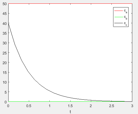
Therefore, the concentration of the reactants
Hence, the concentration of the reactants
Want to see more full solutions like this?
Chapter 28 Solutions
EBK NUMERICAL METHODS FOR ENGINEERS


- For each month of the year, Taylor collected the average high temperatures in Jackson, Mississippi. He used the data to create the histogram shown. Which set of data did he use to create the histogram? A 55, 60, 64, 72, 73, 75, 77, 81, 83, 91, 91, 92\ 55,\ 60,\ 64,\ 72,\ 73,\ 75,\ 77,\ 81,\ 83,\ 91,\ 91,\ 92 55, 60, 64, 72, 73, 75, 77, 81, 83, 91, 91, 92 B 55, 57, 60, 65, 70, 71, 78, 79, 85, 86, 88, 91\ 55,\ 57,\ 60,\ 65,\ 70,\ 71,\ 78,\ 79,\ 85,\ 86,\ 88,\ 91 55, 57, 60, 65, 70, 71, 78, 79, 85, 86, 88, 91 C 55, 60, 63, 64, 65, 71, 83, 87, 88, 88, 89, 93\ 55,\ 60,\ 63,\ 64,\ 65,\ 71,\ 83,\ 87,\ 88,\ 88,\ 89,\ 93 55, 60, 63, 64, 65, 71, 83, 87, 88, 88, 89, 93 D 55, 58, 60, 66, 68, 75, 77, 82, 86, 89, 91, 91\ 55,\ 58,\ 60,\ 66,\ 68,\ 75,\ 77,\ 82,\ 86,\ 89,\ 91,\ 91 55, 58, 60, 66, 68, 75, 77, 82, 86, 89, 91, 91arrow_forward3. Consider the polynomial equation 6-iz+7z2-iz³ +z = 0 for which the roots are 3i, -2i, -i, and i. (a) Verify the relations between this roots and the coefficients of the polynomial. (b) Find the annulus region in which the roots lie.arrow_forwardc) Using only Laplace transforms solve the following Samuelson model given below i.e., the second order difference equation (where yt is national income): - Yt+2 6yt+1+5y₁ = 0, if y₁ = 0 for t < 0, and y₁ = 0, y₁ = 1 1-e-s You may use without proof that L-1[s(1-re-s)] = f(t) = r² for n ≤tarrow_forwardScoring: MATH 15 FILING /10 COMPARISON /10 RULER I 13 Express EMPLOYMENT PROFESSIONALS NAME: SKILLS EVALUATION TEST- Light Industrial MATH-Solve the following problems. (Feel free to use a calculator.) DATE: 1. If you were asked to load 225 boxes onto a truck, and the boxes are crated, with each crate containing nine boxes, how many crates would you need to load? 2. Imagine you live only one mile from work and you decide to walk. If you walk four miles per hour, how long will it take you to walk one mile? 3. Add 3 feet 6 inches + 8 feet 2 inches + 4 inches + 2 feet 5 inches. 4. In a grocery store, steak costs $3.85 per pound. If you buy a three-pound steak and pay for it with a $20 bill, how much change will you get? 5. Add 8 minutes 32 seconds + 37 minutes 18 seconds + 15 seconds. FILING - In the space provided, write the number of the file cabinet where the company should be filed. Example: File Cabinet #4 Elson Co. File Cabinets: 1. Aa-Bb 3. Cg-Dz 5. Ga-Hz 7. La-Md 9. Na-Oz 2. Bc-Cf…arrow_forwardIf you were asked to load 225 boxes onto a truck, and the boxes are crated, with each crate containing nine boxes, how many crates would you need to load?arrow_forwardHabitat for Humanity International is a nonprofit organization dedicated to eliminating poverty housing worldwide. Suppose the following table contains estimates of activity times (in days) involved in the construction of a house that Habitat for Humanity is building. Activity Optimistic Most Probable Pessimistic A 6 7.0 8 B 7 8.0 9 C 7 7.5 11.5 D 7 9.0 10 E 6 7.0 9 F 3 4.0 5 (a) Compute the expected activity completion times and the variance for each activity. (Round your answers to two decimal places.) Activity Expected Times A B C D E F Variance (b) An analyst determined that the critical path consists of activities B-D-F. Compute the expected project completion time and the variance of this path. (Round your answers to two decimal places.) expected project completion time variance of projection completion timearrow_forwardTo manage the production of an animated movie, Pixar Animation Studios has listed the major activities involved, the predecessor relationships, and activity times (in months). The project is completed when activities F and G are both complete. Activity Immediate Predecessor G A B CD E A A C, B C, B D, E Time 4 6 2 6 3 3 5 (a) Find the critical path. (Enter your answers as a comma-separated list.) (b) The project must be completed in 1.5 years. Do you anticipate difficulty in meeting the deadline? Explain. The critical path activities require months to complete. Thus the project ---Select--- be completed in 1.5 years.arrow_forwardTo help with preparations, a couple has devised a project network to describe the activities that must be completed by their wedding date. In addition, they have estimated the time of each activity (in weeks). Start D F B E G Activity A B C DEFGH Time 5 3 6 6 6 3 11 10 (a) Identify the critical path. (Enter your answers as a comma-separated list.) H Finish (b) How much time (in weeks) will be needed to complete this project? week(s) (c) Can activity D be delayed without delaying the entire project? If so, by how many weeks? (If the activity can not be delayed, enter 0.) week(s) (d) Can activity C be delayed without delaying the entire project? If so, by how many weeks? (If the activity can not be delayed, enter 0.) week(s) (e) What is the schedule for activity E (in weeks)? Earliest Start Latest Start Earliest Finish Latest Finish week(s) week(s) week(s) week(s)arrow_forward30.6. Classify the zeros and singularities of the functions tanz (a). f(z)=sin(1-2-1), (b). f(2) = (c). f(z)= tanh .arrow_forward1. Locate the singularities of three of the following functions, and determine their type. (a) f(z)=2(z-sinz). (b) f(z) = (-) (c) f(z) = (z+2-22²)-1 (d) f(z) = sinzarrow_forwardQ 2/classify the zeros and poles of the function f(z) = tanz Zarrow_forward30.1. Show that z = 0 is a removable singularity of the following functions. Furthermore, define f(0) such that these functions are analytic at z = 0. (a). f(z) = 2 sin z- z 1-12² - cos z (b). f(z) = (c). f(z) = sin 22arrow_forwardarrow_back_iosSEE MORE QUESTIONSarrow_forward_ios
 Glencoe Algebra 1, Student Edition, 9780079039897...AlgebraISBN:9780079039897Author:CarterPublisher:McGraw Hill
 College AlgebraAlgebraISBN:9781305115545Author:James Stewart, Lothar Redlin, Saleem WatsonPublisher:Cengage Learning
 Algebra and Trigonometry (MindTap Course List)AlgebraISBN:9781305071742Author:James Stewart, Lothar Redlin, Saleem WatsonPublisher:Cengage Learning