
Concept explainers
Videos
The basic differential equation of the elastic curve for a uniformly loaded beam (Fig. P28.27) is given as
Where
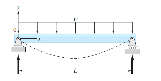
FIGURE P28.27
(a)
To calculate: The deflection of the beam by the finite-difference method with
Answer to Problem 27P
Solution:
The deflection of the beam by the finite-difference method is,
| x | y | y-Analytical |
| 0 | 0 | 0 |
| 24 | ||
| 48 | ||
| 72 | ||
| 96 | ||
| 120 | 0 | 0 |
Explanation of Solution
Given Information:
The differential equation for the elastic curve for a uniformly loaded beam is given as,
Formula to find analytical value,
Where,
The modulus of elasticity,
The moment of inertia,
The values,
Formula used:
The conversion formula,
The value of second order derivative by finite difference method is given as,
Calculation:
Consider the equation,
Rewrite the above equation as,
Substitute the values,
Now, the second order derivative by finite difference method gives,
Therefore,
Put
The boundary condition is,
Put
Substitute
Put
Substitute
Put
Substitute
The matrix form of the above equations is given as below,
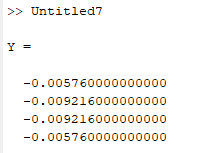
Use MATLAB to find the solution of the above system as below,
Code:
%Write the matrix
A=[-2 1 0 0; 1 -2 1 0; 0 1 -2 1; 0 0 1 -2];
%write the values of rhs
b=[0.002304 0.003456 0.003456 0.002304]';
%find the result
Y=A\b
Output:
Now, for the analytical value, consider the equation
Substitute the values,
Use excel to find the values of y at different values of x as below,
Step 1: Name the column A as x and go to column A2 and put 0 then go to column A3 and write the formula as,
=A2+24
Then, Press enter and drag the column up to
Step 2: Now name the column B as y and go to column B2 andwrite the formula as,
=2.89236*10^(-10)*A2*(120*A2^2-0.5*A2^3-864000)
Step 3: Press enter and drag the column up to
The result obtained as,
| x | y-Analytical |
| 0 | 0 |
| 24 | |
| 48 | |
| 72 | |
| 96 | |
| 120 | 0 |
(b)
To calculate: The deflection of the beam by the shooting method with
Answer to Problem 27P
Solution:
A few values of deflection of the beam by the shooting method is,
| x | y | z |
| 0 | 0 | -1.6E-06 |
| 0.25 | -4.1E-07 | -1.6E-06 |
| 0.5 | -8.2E-07 | -1.6E-06 |
| 0.75 | -1.2E-06 | -1.6E-06 |
| 1 | -1.6E-06 | -1.6E-06 |
| 1.25 | -2E-06 | -1.5E-06 |
| 1.5 | -2.4E-06 | -1.4E-06 |
| 1.75 | -2.8E-06 | -1.4E-06 |
| 2 | -3.2E-06 | -1.3E-06 |
| 2.25 | -3.5E-06 | -1.2E-06 |
| 2.5 | -3.8E-06 | -1.1E-06 |
| 2.75 | -4.1E-06 | -1E-06 |
| 3 | -4.4E-06 | -9E-07 |
Explanation of Solution
Given Information:
The differential equation for the elastic curve for a uniformly loaded beam is given as,
Formula to find analytical value,
Where,
The modulus of elasticity,
The moment of inertia,
The values,
Formula used:
The conversion formula,
Calculation:
Consider the equation,
Rewrite the equation as,
Assume
Substitute the values,
Use VBA program as below to solve the above differential equation as below,
Code:
OptionExplicit
'Create a function find
Subfind()
'declare the variables as integer
Dim n AsInteger, j AsInteger
'declare the variables as double
DimdydxAsDouble, x AsDouble, dy2dx AsDouble, yanalAsDouble, E AsDouble, I AsDouble, w AsDouble, L AsDouble
DimolddydxAsDouble, oldy AsDouble, y AsDouble, h AsDouble
'Set the values of the variables
E =30000
I =800
w =1
L =10
y =0
x =0
h =0.25
dydx=0
'store dydx and analytical solution
dydx= caldydx(w, E, I, L, x)
yanal= caly(w, E, I, L, x)
'use for loop to determine different value of y and y analytical
For j =1 To41
'store the value of y at oldy and dydx in olddydx
oldy = y
olddydx= dydx
'Store d2ydx, dydx and analytical solution
dy2dx = caldy2dx(w, E, I, L, x)
dydx= caldydx(w, E, I, L, x)
yanal= caly(w, E, I, L, x)
'move to the cell b3
Range("b1"). Select
ActiveCell.Value="shooting method"
'Assign name to the columns
ActiveCell.Offset(1,0). Select
ActiveCell.Value="x"
ActiveCell.Offset(0,1). Select
ActiveCell.Value="y"
ActiveCell.Offset(0,1). Select
ActiveCell.Value="z"
ActiveCell.Offset(0,1). Select
ActiveCell.Value="dy2dx"
ActiveCell.Offset(0,1). Select
ActiveCell.Value="y-anal"
'dislay values in cell
Range("b2"). Select
ActiveCell.Offset(j,0). Select
ActiveCell.Value= x
ActiveCell.Offset(0,1). Select
ActiveCell.Value= oldy
ActiveCell.Offset(0,1). Select
ActiveCell.Value= dydx
ActiveCell.Offset(0,1). Select
ActiveCell.Value= dy2dx
ActiveCell.Offset(0,1). Select
ActiveCell.Value= yanal
'Write the next value of x
x = x + h
'Write the next value of y by euler method
y = oldy + olddydx* h
Next
EndSub
'Define d2ydx function
Function caldy2dx(w, E, I, L, x)
'Declare the variables
Dim t AsDouble
'Write the formula
t =((w * L * x)/(2* E * I))-((w * x * x)/(2* E * I))
'Store the value
caldy2dx = t
EndFunction
'Define dydx
Functioncaldydx(w, E, I, L, x)
'Declare the variables
Dim t AsDouble, c AsDouble
'Set the values
c =-0.000001648
'Write the formula
t =((w * L * x * x)/(4* E * I))-((w * x * x * x)/(6* E * I))+ c
'Store the value
caldydx= t
EndFunction
'Define the function caly for analytical value
Functioncaly(w, E, I, L, x)
'Declare the variables
Dim t AsDouble
'Write the formula
t =((w * L * x * x * x)/(12* E * I))-((w * x * x * x * x)/(24* E * I))-((w * L * L * L * x)/(24* E * I))
'Store the value
caly= t
EndFunction
Output:
| shooting method | ||||
| x | y | z | dy2dx | y-anal |
| 0 | 0 | -1.6E-06 | 0 | 0 |
| 0.25 | -4.1E-07 | -1.6E-06 | 5.08E-08 | -4.3E-07 |
| 0.5 | -8.2E-07 | -1.6E-06 | 9.9E-08 | -8.6E-07 |
| 0.75 | -1.2E-06 | -1.6E-06 | 1.45E-07 | -1.3E-06 |
| 1 | -1.6E-06 | -1.6E-06 | 1.88E-07 | -1.7E-06 |
| 1.25 | -2E-06 | -1.5E-06 | 2.28E-07 | -2.1E-06 |
| 1.5 | -2.4E-06 | -1.4E-06 | 2.66E-07 | -2.5E-06 |
| 1.75 | -2.8E-06 | -1.4E-06 | 3.01E-07 | -2.9E-06 |
| 2 | -3.2E-06 | -1.3E-06 | 3.33E-07 | -3.2E-06 |
| 2.25 | -3.5E-06 | -1.2E-06 | 3.63E-07 | -3.6E-06 |
| 2.5 | -3.8E-06 | -1.1E-06 | 3.91E-07 | -3.9E-06 |
| 2.75 | -4.1E-06 | -1E-06 | 4.15E-07 | -4.2E-06 |
| 3 | -4.4E-06 | -9E-07 | 4.38E-07 | -4.4E-06 |
| 3.25 | -4.7E-06 | -7.9E-07 | 4.57E-07 | -4.6E-06 |
| 3.5 | -4.9E-06 | -6.7E-07 | 4.74E-07 | -4.8E-06 |
| 3.75 | -5.1E-06 | -5.5E-07 | 4.88E-07 | -5E-06 |
| 4 | -5.2E-06 | -4.3E-07 | 5E-07 | -5.2E-06 |
| 4.25 | -5.4E-06 | -3E-07 | 5.09E-07 | -5.3E-06 |
| 4.5 | -5.5E-06 | -1.7E-07 | 5.16E-07 | -5.4E-06 |
| 4.75 | -5.6E-06 | -4.2E-08 | 5.2E-07 | -5.4E-06 |
| 5 | -5.6E-06 | 8.81E-08 | 5.21E-07 | -5.4E-06 |
| 5.25 | -5.6E-06 | 2.18E-07 | 5.2E-07 | -5.4E-06 |
| 5.5 | -5.6E-06 | 3.48E-07 | 5.16E-07 | -5.4E-06 |
| 5.75 | -5.5E-06 | 4.76E-07 | 5.09E-07 | -5.3E-06 |
| 6 | -5.4E-06 | 6.02E-07 | 5E-07 | -5.2E-06 |
| 6.25 | -5.3E-06 | 7.26E-07 | 4.88E-07 | -5E-06 |
| 6.5 | -5.2E-06 | 8.46E-07 | 4.74E-07 | -4.8E-06 |
| 6.75 | -5E-06 | 9.62E-07 | 4.57E-07 | -4.6E-06 |
| 7 | -4.8E-06 | 1.07E-06 | 4.38E-07 | -4.4E-06 |
| 7.25 | -4.5E-06 | 1.18E-06 | 4.15E-07 | -4.2E-06 |
| 7.5 | -4.3E-06 | 1.28E-06 | 3.91E-07 | -3.9E-06 |
| 7.75 | -4E-06 | 1.38E-06 | 3.63E-07 | -3.6E-06 |
| 8 | -3.7E-06 | 1.46E-06 | 3.33E-07 | -3.2E-06 |
| 8.25 | -3.3E-06 | 1.54E-06 | 3.01E-07 | -2.9E-06 |
| 8.5 | -3E-06 | 1.61E-06 | 2.66E-07 | -2.5E-06 |
| 8.75 | -2.6E-06 | 1.68E-06 | 2.28E-07 | -2.1E-06 |
| 9 | -2.2E-06 | 1.73E-06 | 1.88E-07 | -1.7E-06 |
| 9.25 | -1.7E-06 | 1.77E-06 | 1.45E-07 | -1.3E-06 |
| 9.5 | -1.3E-06 | 1.8E-06 | 9.9E-08 | -8.6E-07 |
| 9.75 | -8.7E-07 | 1.82E-06 | 5.08E-08 | -4.3E-07 |
| 10 | -4.2E-07 | 1.82E-06 | 0 | 0 |
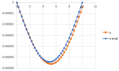
Now, to draw the graph of y and y-analytical follow the step as below,
Step 1: Select the cell from B2 to B43 and cell C2 to C43. Then, go to the Insert and select the scatter with smooth lines from the chart.
Step 2: Select the cell from B2 to B43 and cell F2 to F43. Then, go to the Insert and select the scatter with smooth lines from the chart.
Step 3: Select one of the graphs and paste it on another graph to merge the graphs.
The graph obtained is,
Want to see more full solutions like this?
Chapter 28 Solutions
EBK NUMERICAL METHODS FOR ENGINEERS
Additional Engineering Textbook Solutions
Probability And Statistical Inference (10th Edition)
Introductory Statistics
Finite Mathematics for Business, Economics, Life Sciences and Social Sciences
Elementary and Intermediate Algebra: Concepts and Applications (7th Edition)
A First Course in Probability (10th Edition)
Precalculus: A Unit Circle Approach (3rd Edition)


- Problem (14): A pump is being used to lift water from an underground tank through a pipe of diameter (d) at discharge (Q). The total head loss until the pump entrance can be calculated as (h₁ = K[V²/2g]), h where (V) is the flow velocity in the pipe. The elevation difference between the pump and tank surface is (h). Given the values of h [cm], d [cm], and K [-], calculate the maximum discharge Q [Lit/s] beyond which cavitation would take place at the pump entrance. Assume Turbulent flow conditions. Givens: h = 120.31 cm d = 14.455 cm K = 8.976 Q Answers: (1) 94.917 lit/s (2) 49.048 lit/s ( 3 ) 80.722 lit/s 68.588 lit/s 4arrow_forwardProblem (13): A pump is being used to lift water from the bottom tank to the top tank in a galvanized iron pipe at a discharge (Q). The length and diameter of the pipe section from the bottom tank to the pump are (L₁) and (d₁), respectively. The length and diameter of the pipe section from the pump to the top tank are (L2) and (d2), respectively. Given the values of Q [L/s], L₁ [m], d₁ [m], L₂ [m], d₂ [m], calculate total head loss due to friction (i.e., major loss) in the pipe (hmajor-loss) in [cm]. Givens: L₁,d₁ Pump L₂,d2 오 0.533 lit/s L1 = 6920.729 m d1 = 1.065 m L2 = 70.946 m d2 0.072 m Answers: (1) 3.069 cm (2) 3.914 cm ( 3 ) 2.519 cm ( 4 ) 1.855 cm TABLE 8.1 Equivalent Roughness for New Pipes Pipe Riveted steel Concrete Wood stave Cast iron Galvanized iron Equivalent Roughness, & Feet Millimeters 0.003-0.03 0.9-9.0 0.001-0.01 0.3-3.0 0.0006-0.003 0.18-0.9 0.00085 0.26 0.0005 0.15 0.045 0.000005 0.0015 0.0 (smooth) 0.0 (smooth) Commercial steel or wrought iron 0.00015 Drawn…arrow_forwardThe flow rate is 12.275 Liters/s and the diameter is 6.266 cm.arrow_forward
- An experimental setup is being built to study the flow in a large water main (i.e., a large pipe). The water main is expected to convey a discharge (Qp). The experimental tube will be built at a length scale of 1/20 of the actual water main. After building the experimental setup, the pressure drop per unit length in the model tube (APm/Lm) is measured. Problem (20): Given the value of APm/Lm [kPa/m], and assuming pressure coefficient similitude, calculate the drop in the pressure per unit length of the water main (APP/Lp) in [Pa/m]. Givens: AP M/L m = 590.637 kPa/m meen Answers: ( 1 ) 59.369 Pa/m ( 2 ) 73.83 Pa/m (3) 95.443 Pa/m ( 4 ) 44.444 Pa/m *******arrow_forwardFind the reaction force in y if Ain = 0.169 m^2, Aout = 0.143 m^2, p_in = 0.552 atm, Q = 0.367 m^3/s, α = 31.72 degrees. The pipe is flat on the ground so do not factor in weight of the pipe and fluid.arrow_forwardFind the reaction force in x if Ain = 0.301 m^2, Aout = 0.177 m^2, p_in = 1.338 atm, Q = 0.669 m^3/s, and α = 37.183 degreesarrow_forward
- Problem 5: Three-Force Equilibrium A structural connection at point O is in equilibrium under the action of three forces. • • . Member A applies a force of 9 kN vertically upward along the y-axis. Member B applies an unknown force F at the angle shown. Member C applies an unknown force T along its length at an angle shown. Determine the magnitudes of forces F and T required for equilibrium, assuming 0 = 90° y 9 kN Aarrow_forwardProblem 19: Determine the force in members HG, HE, and DE of the truss, and state if the members are in tension or compression. 4 ft K J I H G B C D E F -3 ft -3 ft 3 ft 3 ft 3 ft- 1500 lb 1500 lb 1500 lb 1500 lb 1500 lbarrow_forwardProblem 14: Determine the reactions at the pin A, and the tension in cord. Neglect the thickness of the beam. F1=26kN F2 13 12 80° -2m 3marrow_forward
- Problem 22: Determine the force in members GF, FC, and CD of the bridge truss and state if the members are in tension or compression. F 15 ft B D -40 ft 40 ft -40 ft 40 ft- 5 k 10 k 15 k 30 ft Earrow_forwardProblem 20: Determine the force in members BC, HC, and HG. After the truss is sectioned use a single equation of equilibrium for the calculation of each force. State if the members are in tension or compression. 5 kN 4 kN 4 kN 3 kN 2 kN B D E F 3 m -5 m- -5 m- 5 m 5 m-arrow_forwardAn experimental setup is being built to study the flow in a large water main (i.e., a large pipe). The water main is expected to convey a discharge (Qp). The experimental tube will be built at a length scale of 1/20 of the actual water main. After building the experimental setup, the pressure drop per unit length in the model tube (APm/Lm) is measured. Problem (19): Given the value of Qp [m³/s], and assuming Reynolds number similitude between the water main and experimental tube, calculate the flow rate in the model tube (Qm) in [lit/s]. = 30.015 m^3/sarrow_forward
 Elements Of ElectromagneticsMechanical EngineeringISBN:9780190698614Author:Sadiku, Matthew N. O.Publisher:Oxford University Press
 Mechanics of Materials (10th Edition)Mechanical EngineeringISBN:9780134319650Author:Russell C. HibbelerPublisher:PEARSON
 Thermodynamics: An Engineering ApproachMechanical EngineeringISBN:9781259822674Author:Yunus A. Cengel Dr., Michael A. BolesPublisher:McGraw-Hill Education
 Control Systems EngineeringMechanical EngineeringISBN:9781118170519Author:Norman S. NisePublisher:WILEY
 Mechanics of Materials (MindTap Course List)Mechanical EngineeringISBN:9781337093347Author:Barry J. Goodno, James M. GerePublisher:Cengage Learning
 Engineering Mechanics: StaticsMechanical EngineeringISBN:9781118807330Author:James L. Meriam, L. G. Kraige, J. N. BoltonPublisher:WILEY