Fundamentals of Statistics (5th Edition)
5th Edition
ISBN: 9780134508306
Author: Michael Sullivan III
Publisher: PEARSON
expand_more
expand_more
format_list_bulleted
Videos
Textbook Question
Chapter 2.3, Problem 15AYU
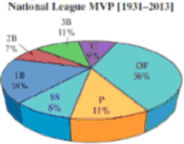
National League Baseball MVP The following pie chart displays the position played by the most valuable player (MVP) in the National League of Major League Baseball from 1931 thru 2013. Explain how the graphic is misleading. What should be done to improve the graphic?
Expert Solution & Answer
Want to see the full answer?
Check out a sample textbook solution
Students have asked these similar questions
Find binomial probability if:
x = 8, n = 10, p = 0.7
x= 3, n=5, p = 0.3
x = 4, n=7, p = 0.6
Quality Control: A factory produces light bulbs with a 2% defect rate. If a random sample of 20 bulbs is tested, what is the probability that exactly 2 bulbs are defective? (hint: p=2% or 0.02; x =2, n=20; use the same logic for the following problems)
Marketing Campaign: A marketing company sends out 1,000 promotional emails. The probability of any email being opened is 0.15. What is the probability that exactly 150 emails will be opened? (hint: total emails or n=1000, x =150)
Customer Satisfaction: A survey shows that 70% of customers are satisfied with a new product. Out of 10 randomly selected customers, what is the probability that at least 8 are satisfied? (hint: One of the keyword in this question is “at least 8”, it is not “exactly 8”, the correct formula for this should be = 1- (binom.dist(7, 10, 0.7, TRUE)). The part in the princess will give you the probability of seven and less than…
please answer these questions
Selon une économiste d’une société financière, les dépenses moyennes pour « meubles et appareils de maison » ont été moins importantes pour les ménages de la région de Montréal, que celles de la région de Québec.
Un échantillon aléatoire de 14 ménages pour la région de Montréal et de 16 ménages pour la région Québec est tiré et donne les données suivantes, en ce qui a trait aux dépenses pour ce secteur d’activité économique.
On suppose que les données de chaque population sont distribuées selon une loi normale.
Nous sommes intéressé à connaitre si les variances des populations sont égales.a) Faites le test d’hypothèse sur deux variances approprié au seuil de signification de 1 %. Inclure les informations suivantes :
i. Hypothèse / Identification des populationsii. Valeur(s) critique(s) de Fiii. Règle de décisioniv. Valeur du rapport Fv. Décision et conclusion
b) A partir des résultats obtenus en a), est-ce que l’hypothèse d’égalité des variances pour cette…
Chapter 2 Solutions
Fundamentals of Statistics (5th Edition)
Ch. 2.1 - Define raw data in your own words.Ch. 2.1 - A frequency distribution lists the _____ of...Ch. 2.1 - In a relative frequency distribution, what should...Ch. 2.1 - What is a bar graph? What is a Pareto chart?Ch. 2.1 - Flu Season The pie chart shown, the type we see in...Ch. 2.1 - Cosmetic Surgery This USA Today type chart shows...Ch. 2.1 - Most Valuable Player The following Pareto chart...Ch. 2.1 - Poverty The U.S. Census Bureau uses money income...Ch. 2.1 - Divorce The following graph represents the results...Ch. 2.1 - Identity Theft Identity fraud occurs when someone...
Ch. 2.1 - Made in America A random sample of 2163 adults...Ch. 2.1 - Desirability Attributes A random sample of 2163...Ch. 2.1 - College Survey In a national survey conducted by...Ch. 2.1 - College Survey In a national survey conducted by...Ch. 2.1 - Use the Internet? The Gallup organization...Ch. 2.1 - Dining Out A sample of 521 adults was asked, How...Ch. 2.1 - NW Texting A survey of U.S. adults and teens (ages...Ch. 2.1 - Educational Attainment The educational attainment...Ch. 2.1 - Dream Job A survey of adult men and women asked,...Ch. 2.1 - Car Color A survey of 100 randomly selected autos...Ch. 2.1 - Prob. 21AYUCh. 2.1 - Bachelor Party In a survey conducted by Opinion...Ch. 2.1 - Favorite Day to Eat Out A survey was conducted by...Ch. 2.1 - Prob. 25AYUCh. 2.1 - Prob. 26AYUCh. 2.1 - Prob. 27AYUCh. 2.1 - StatCrunch Survey Choose a qualitative variable...Ch. 2.1 - Putting It Together: Online Homework Keeping...Ch. 2.1 - When should relative frequencies be used when...Ch. 2.1 - Prob. 31AYUCh. 2.1 - Prob. 32AYUCh. 2.1 - Prob. 33AYUCh. 2.2 - The categories by which data are grouped are...Ch. 2.2 - The _____ class limit is the smallest value within...Ch. 2.2 - The _____ is the difference between consecutive...Ch. 2.2 - Prob. 4AYUCh. 2.2 - Prob. 5AYUCh. 2.2 - Prob. 6AYUCh. 2.2 - True or False: The shape of the distribution shown...Ch. 2.2 - Prob. 8AYUCh. 2.2 - Rolling the Dice An experiment was conducted in...Ch. 2.2 - Car Sales A car salesman records the number of...Ch. 2.2 - IQ Scores The following frequency histogram...Ch. 2.2 - Alcohol-Related Traffic Fatalities The frequency...Ch. 2.2 - In Problems 13 and 14, for each variable...Ch. 2.2 - In Problems 13 and 14, for each variable...Ch. 2.2 - Misery Index The following time-series plot shows...Ch. 2.2 - Prob. 16AYUCh. 2.2 - Predicting School Enrollment To predict future...Ch. 2.2 - Free Throws In an experiment, a researcher asks a...Ch. 2.2 - In Problems 1922, determine the original set of...Ch. 2.2 - In Problems 1922, determine the original set of...Ch. 2.2 - In Problems 1922, determine the original set of...Ch. 2.2 - In Problems 1922, determine the original set of...Ch. 2.2 - find (a) the number of classes, (b) the class...Ch. 2.2 - Earthquakes The following data represent the...Ch. 2.2 - In Problems 25 and 26, construct (a) a relative...Ch. 2.2 - In Problems 25 and 26, construct (a) a relative...Ch. 2.2 - NW Televisions in the Household A researcher with...Ch. 2.2 - Waiting The data below represent the number of...Ch. 2.2 - NW Gini Index The Gini Index is a measure of how...Ch. 2.2 - Average Income The following data represent the...Ch. 2.2 - Cigarette Tex Rates The table shows the tax, in...Ch. 2.2 - Dividend Yield A dividend is a payment from a...Ch. 2.2 - NW Violent Crimes Violent crimes include murder,...Ch. 2.2 - Volume of Altria Group Stock The volume of a stock...Ch. 2.2 - Prob. 35AYUCh. 2.2 - Prob. 36AYUCh. 2.2 - Prob. 37AYUCh. 2.2 - Prob. 38AYUCh. 2.2 - Prob. 39AYUCh. 2.2 - Prob. 40AYUCh. 2.2 - NW Violent Crimes Use the violent crime rate data...Ch. 2.2 - Academy Award Winners The following data represent...Ch. 2.2 - Prob. 43AYUCh. 2.2 - Sullivan Survey Choose a continuous quantitative...Ch. 2.2 - Prob. 46AYUCh. 2.2 - Prob. 47AYUCh. 2.2 - Waiting Draw a dot plot of the waiting data from...Ch. 2.2 - Prob. 49AYUCh. 2.2 - Prob. 50AYUCh. 2.2 - Prob. 51AYUCh. 2.2 - Prob. 52AYUCh. 2.2 - Prob. 53AYUCh. 2.2 - Putting It Together: Which Graphical Summary?...Ch. 2.2 - Prob. 55AYUCh. 2.2 - Prob. 56AYUCh. 2.2 - Discuss the advantages and disadvantages of...Ch. 2.2 - Prob. 58AYUCh. 2.2 - Describe the situations in which it is preferable...Ch. 2.2 - Sketch four histogramsone skewed right, one skewed...Ch. 2.2 - What type of variable is required when drawing...Ch. 2.3 - Inauguration Cost The following is a USA...Ch. 2.3 - Burning Calories The following is a USA Today-type...Ch. 2.3 - NW Median Earnings The graph shows the median...Ch. 2.3 - Union Membership The following relative frequency...Ch. 2.3 - NW Robberies A newspaper article claimed that the...Ch. 2.3 - Car Accidents An article in a student newspaper...Ch. 2.3 - Tax Revenue The following histogram drawn in...Ch. 2.3 - You Explain It! Oil Reserves The U.S. Strategic...Ch. 2.3 - NW Cost of Kids The following is a USA Today-type...Ch. 2.3 - Worker Injury The safety manager at Klutz...Ch. 2.3 - Health Care Expenditures The following data...Ch. 2.3 - Prob. 12AYUCh. 2.3 - NW Overweight Between 1980 and 2012, the number of...Ch. 2.3 - Ideal Family Size The following USA Today-type...Ch. 2.3 - National League Baseball MVP The following pie...Ch. 2.3 - Prob. 16AYUCh. 2 - Effective Commercial Harris Interactive conducted...Ch. 2 - Weapons Used in Homicide The following frequency...Ch. 2 - Live Births The following frequency distribution...Ch. 2 - Political Affiliation One hundred randomly...Ch. 2 - Family Size A random sample of 60 couples married...Ch. 2 - Home Ownership Rates The table shows the home...Ch. 2 - Diameter of a Cookie The following data represent...Ch. 2 - Time Online The following data represent the...Ch. 2 - Grade Inflation The side-by-side bar graph to the...Ch. 2 - Income Distribution The following data represent...Ch. 2 - Misleading Graphs In 2013, the average earnings of...Ch. 2 - High Heels The graphic to the right is a USA Today...Ch. 2 - The graph shows the ratings on Yelp for Hot Dougs...Ch. 2 - A random sample of 1005 adult Americans was asked,...Ch. 2 - Interested in knowing the educational background...Ch. 2 - The following data represent the number of cars...Ch. 2 - Dr. Paul Oswiecmiski randomly selects 40 of his...Ch. 2 - The following data represent the time (in minutes)...Ch. 2 - The data below shows birth rate and per capita...Ch. 2 - The following is a USA Today-type graph. Do you...Ch. 2 - A bar graph or pie chart (or both) that depicts...Ch. 2 - A histogram that displays the distribution of...Ch. 2 - Six histograms displaying tornado duration for...Ch. 2 - A bar chart that shows the relationship between...Ch. 2 - A bar chart that shows the relationship between...Ch. 2 - A general summary of your findings and...
Knowledge Booster


Learn more about
Need a deep-dive on the concept behind this application? Look no further. Learn more about this topic, statistics and related others by exploring similar questions and additional content below.Similar questions
- According to an economist from a financial company, the average expenditures on "furniture and household appliances" have been lower for households in the Montreal area than those in the Quebec region. A random sample of 14 households from the Montreal region and 16 households from the Quebec region was taken, providing the following data regarding expenditures in this economic sector. It is assumed that the data from each population are distributed normally. We are interested in knowing if the variances of the populations are equal. a) Perform the appropriate hypothesis test on two variances at a significance level of 1%. Include the following information: i. Hypothesis / Identification of populations ii. Critical F-value(s) iii. Decision rule iv. F-ratio value v. Decision and conclusion b) Based on the results obtained in a), is the hypothesis of equal variances for this socio-economic characteristic measured in these two populations upheld? c) Based on the results obtained in a),…arrow_forwardA major company in the Montreal area, offering a range of engineering services from project preparation to construction execution, and industrial project management, wants to ensure that the individuals who are responsible for project cost estimation and bid preparation demonstrate a certain uniformity in their estimates. The head of civil engineering and municipal services decided to structure an experimental plan to detect if there could be significant differences in project evaluation. Seven projects were selected, each of which had to be evaluated by each of the two estimators, with the order of the projects submitted being random. The obtained estimates are presented in the table below. a) Complete the table above by calculating: i. The differences (A-B) ii. The sum of the differences iii. The mean of the differences iv. The standard deviation of the differences b) What is the value of the t-statistic? c) What is the critical t-value for this test at a significance level of 1%?…arrow_forwardCompute the relative risk of falling for the two groups (did not stop walking vs. did stop). State/interpret your result verbally.arrow_forward
- Microsoft Excel include formulasarrow_forwardQuestion 1 The data shown in Table 1 are and R values for 24 samples of size n = 5 taken from a process producing bearings. The measurements are made on the inside diameter of the bearing, with only the last three decimals recorded (i.e., 34.5 should be 0.50345). Table 1: Bearing Diameter Data Sample Number I R Sample Number I R 1 34.5 3 13 35.4 8 2 34.2 4 14 34.0 6 3 31.6 4 15 37.1 5 4 31.5 4 16 34.9 7 5 35.0 5 17 33.5 4 6 34.1 6 18 31.7 3 7 32.6 4 19 34.0 8 8 33.8 3 20 35.1 9 34.8 7 21 33.7 2 10 33.6 8 22 32.8 1 11 31.9 3 23 33.5 3 12 38.6 9 24 34.2 2 (a) Set up and R charts on this process. Does the process seem to be in statistical control? If necessary, revise the trial control limits. [15 pts] (b) If specifications on this diameter are 0.5030±0.0010, find the percentage of nonconforming bearings pro- duced by this process. Assume that diameter is normally distributed. [10 pts] 1arrow_forward4. (5 pts) Conduct a chi-square contingency test (test of independence) to assess whether there is an association between the behavior of the elderly person (did not stop to talk, did stop to talk) and their likelihood of falling. Below, please state your null and alternative hypotheses, calculate your expected values and write them in the table, compute the test statistic, test the null by comparing your test statistic to the critical value in Table A (p. 713-714) of your textbook and/or estimating the P-value, and provide your conclusions in written form. Make sure to show your work. Did not stop walking to talk Stopped walking to talk Suffered a fall 12 11 Totals 23 Did not suffer a fall | 2 Totals 35 37 14 46 60 Tarrow_forward
- Question 2 Parts manufactured by an injection molding process are subjected to a compressive strength test. Twenty samples of five parts each are collected, and the compressive strengths (in psi) are shown in Table 2. Table 2: Strength Data for Question 2 Sample Number x1 x2 23 x4 x5 R 1 83.0 2 88.6 78.3 78.8 3 85.7 75.8 84.3 81.2 78.7 75.7 77.0 71.0 84.2 81.0 79.1 7.3 80.2 17.6 75.2 80.4 10.4 4 80.8 74.4 82.5 74.1 75.7 77.5 8.4 5 83.4 78.4 82.6 78.2 78.9 80.3 5.2 File Preview 6 75.3 79.9 87.3 89.7 81.8 82.8 14.5 7 74.5 78.0 80.8 73.4 79.7 77.3 7.4 8 79.2 84.4 81.5 86.0 74.5 81.1 11.4 9 80.5 86.2 76.2 64.1 80.2 81.4 9.9 10 75.7 75.2 71.1 82.1 74.3 75.7 10.9 11 80.0 81.5 78.4 73.8 78.1 78.4 7.7 12 80.6 81.8 79.3 73.8 81.7 79.4 8.0 13 82.7 81.3 79.1 82.0 79.5 80.9 3.6 14 79.2 74.9 78.6 77.7 75.3 77.1 4.3 15 85.5 82.1 82.8 73.4 71.7 79.1 13.8 16 78.8 79.6 80.2 79.1 80.8 79.7 2.0 17 82.1 78.2 18 84.5 76.9 75.5 83.5 81.2 19 79.0 77.8 20 84.5 73.1 78.2 82.1 79.2 81.1 7.6 81.2 84.4 81.6 80.8…arrow_forwardName: Lab Time: Quiz 7 & 8 (Take Home) - due Wednesday, Feb. 26 Contingency Analysis (Ch. 9) In lab 5, part 3, you will create a mosaic plot and conducted a chi-square contingency test to evaluate whether elderly patients who did not stop walking to talk (vs. those who did stop) were more likely to suffer a fall in the next six months. I have tabulated the data below. Answer the questions below. Please show your calculations on this or a separate sheet. Did not stop walking to talk Stopped walking to talk Totals Suffered a fall Did not suffer a fall Totals 12 11 23 2 35 37 14 14 46 60 Quiz 7: 1. (2 pts) Compute the odds of falling for each group. Compute the odds ratio for those who did not stop walking vs. those who did stop walking. Interpret your result verbally.arrow_forwardSolve please and thank you!arrow_forward
- 7. In a 2011 article, M. Radelet and G. Pierce reported a logistic prediction equation for the death penalty verdicts in North Carolina. Let Y denote whether a subject convicted of murder received the death penalty (1=yes), for the defendant's race h (h1, black; h = 2, white), victim's race i (i = 1, black; i = 2, white), and number of additional factors j (j = 0, 1, 2). For the model logit[P(Y = 1)] = a + ß₁₂ + By + B²², they reported = -5.26, D â BD = 0, BD = 0.17, BY = 0, BY = 0.91, B = 0, B = 2.02, B = 3.98. (a) Estimate the probability of receiving the death penalty for the group most likely to receive it. [4 pts] (b) If, instead, parameters used constraints 3D = BY = 35 = 0, report the esti- mates. [3 pts] h (c) If, instead, parameters used constraints Σ₁ = Σ₁ BY = Σ; B = 0, report the estimates. [3 pts] Hint the probabilities, odds and odds ratios do not change with constraints.arrow_forwardSolve please and thank you!arrow_forwardSolve please and thank you!arrow_forward
arrow_back_ios
SEE MORE QUESTIONS
arrow_forward_ios
Recommended textbooks for you
 Holt Mcdougal Larson Pre-algebra: Student Edition...AlgebraISBN:9780547587776Author:HOLT MCDOUGALPublisher:HOLT MCDOUGAL
 Glencoe Algebra 1, Student Edition, 9780079039897...AlgebraISBN:9780079039897Author:CarterPublisher:McGraw Hill
 Elementary Geometry For College Students, 7eGeometryISBN:9781337614085Author:Alexander, Daniel C.; Koeberlein, Geralyn M.Publisher:Cengage,
 Algebra: Structure And Method, Book 1AlgebraISBN:9780395977224Author:Richard G. Brown, Mary P. Dolciani, Robert H. Sorgenfrey, William L. ColePublisher:McDougal Littell
Holt Mcdougal Larson Pre-algebra: Student Edition...
Algebra
ISBN:9780547587776
Author:HOLT MCDOUGAL
Publisher:HOLT MCDOUGAL
Glencoe Algebra 1, Student Edition, 9780079039897...
Algebra
ISBN:9780079039897
Author:Carter
Publisher:McGraw Hill
Elementary Geometry For College Students, 7e
Geometry
ISBN:9781337614085
Author:Alexander, Daniel C.; Koeberlein, Geralyn M.
Publisher:Cengage,
Algebra: Structure And Method, Book 1
Algebra
ISBN:9780395977224
Author:Richard G. Brown, Mary P. Dolciani, Robert H. Sorgenfrey, William L. Cole
Publisher:McDougal Littell
2.1 Introduction to inequalities; Author: Oli Notes;https://www.youtube.com/watch?v=D6erN5YTlXE;License: Standard YouTube License, CC-BY
GCSE Maths - What are Inequalities? (Inequalities Part 1) #56; Author: Cognito;https://www.youtube.com/watch?v=e_tY6X5PwWw;License: Standard YouTube License, CC-BY
Introduction to Inequalities | Inequality Symbols | Testing Solutions for Inequalities; Author: Scam Squad Math;https://www.youtube.com/watch?v=paZSN7sV1R8;License: Standard YouTube License, CC-BY