
Concept explainers
Videos
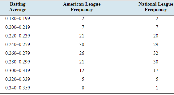
Batting average: The following frequency distribution presents the batting averages of Major League Baseball players in both the American League and the National League who had 300 or more plate appearances during a recent season.
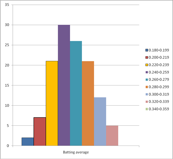
- Construct a frequency histogram for the American League.
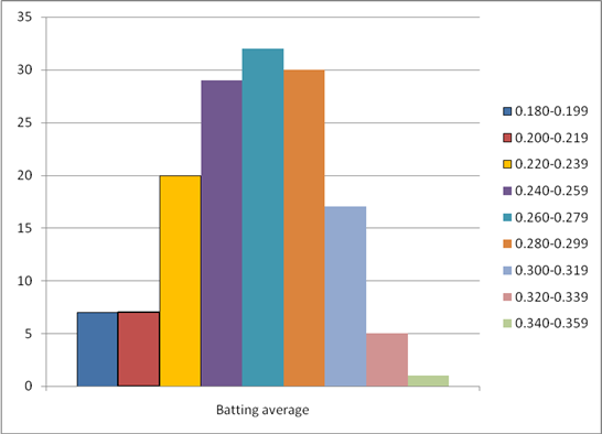
- Construct a frequency histogram for the National League.
- Construct a relative frequency distribution for the American League.
- Construct a relative frequency distribution for the National League.
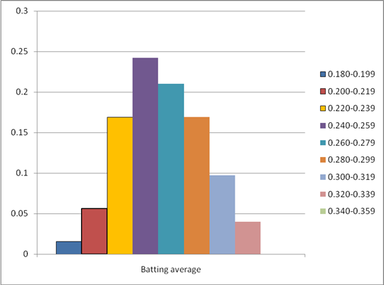
- Construct a relative frequency histogram for the American League.
- Construct a relative frequency histogram for the National League.
- What percentage of American League players had batting averages of 0.300 or more?
- What percentage of National League players had batting averages of 0.300 or more?
- Compare the relative frequency histograms. What is the main difference between the distributions of batting averages in the two leagues?
a.
To construct: A frequency histogram for American League.
Explanation of Solution
Given information:The following frequency distribution presents the batting averages of Major League Baseball players in both the American League and the National League who had 300 or more plate appearances during a recent season.
| Batting average | American LeagueFrequency | National LeagueFrequency |
| 0.180-0.199 | 2 | 2 |
| 0.200-0.219 | 7 | 7 |
| 0.220-0.239 | 21 | 20 |
| 0.240-0.259 | 30 | 29 |
| 0.260-0.279 | 26 | 32 |
| 0.280-0.299 | 21 | 30 |
| 0.300-0.319 | 12 | 17 |
| 0.320-0.339 | 5 | 5 |
| 0.340-0.359 | 0 | 1 |
Definition used: Histograms based on frequency distributions are called frequency histogram.
Solution:
The following frequency distribution presents the batting averages of Major League Baseball players in the American Leaguewho had 300 or more plate appearances during a recent season.
| Batting average | American LeagueFrequency |
| 0.180-0.199 | 2 |
| 0.200-0.219 | 7 |
| 0.220-0.239 | 21 |
| 0.240-0.259 | 30 |
| 0.260-0.279 | 26 |
| 0.280-0.299 | 21 |
| 0.300-0.319 | 12 |
| 0.320-0.339 | 5 |
| 0.340-0.359 | 0 |
The frequency histogram for American League is given by
b.
To construct: A frequency histogram for National League.
Explanation of Solution
Given information:The following frequency distribution presents the batting averages of Major League Baseball players in both the American League and the National League who had 300 or more plate appearances during a recent season.
| Batting average | American LeagueFrequency | National LeagueFrequency |
| 0.180-0.199 | 2 | 2 |
| 0.200-0.219 | 7 | 7 |
| 0.220-0.239 | 21 | 20 |
| 0.240-0.259 | 30 | 29 |
| 0.260-0.279 | 26 | 32 |
| 0.280-0.299 | 21 | 30 |
| 0.300-0.319 | 12 | 17 |
| 0.320-0.339 | 5 | 5 |
| 0.340-0.359 | 0 | 1 |
Definition used: Histograms based on frequency distributions are called frequency histogram.
Solution:
The following frequency distribution presents the batting averages of Major League Baseball players in the American Leaguewho had 300 or more plate appearances during a recent season.
| Batting average | National LeagueFrequency |
| 0.180-0.199 | 2 |
| 0.200-0.219 | 7 |
| 0.220-0.239 | 20 |
| 0.240-0.259 | 29 |
| 0.260-0.279 | 32 |
| 0.280-0.299 | 30 |
| 0.300-0.319 | 17 |
| 0.320-0.339 | 5 |
| 0.340-0.359 | 1 |
The frequency histogram for American League is given by
c.
To construct: A relative frequency distribution for American League.
Explanation of Solution
Given information:The following frequency distribution presents the batting averages of Major League Baseball players in both the American League and the National League who had 300 or more plate appearances during a recent season.
| Batting average | American LeagueFrequency | National LeagueFrequency |
| 0.180-0.199 | 2 | 2 |
| 0.200-0.219 | 7 | 7 |
| 0.220-0.239 | 21 | 20 |
| 0.240-0.259 | 30 | 29 |
| 0.260-0.279 | 26 | 32 |
| 0.280-0.299 | 21 | 30 |
| 0.300-0.319 | 12 | 17 |
| 0.320-0.339 | 5 | 5 |
| 0.340-0.359 | 0 | 1 |
Formula used:
Solution:
From the given table,
The sum of all frequency for American League is
The table of relative frequency is given by
| Batting average | American LeagueFrequency | American LeagueRelative frequency |
| 0.180-0.199 | 2 | |
| 0.200-0.219 | 7 | |
| 0.220-0.239 | 21 | |
| 0.240-0.259 | 30 | |
| 0.260-0.279 | 26 | |
| 0.280-0.299 | 21 | |
| 0.300-0.319 | 12 | |
| 0.320-0.339 | 5 | |
| 0.340-0.359 | 0 |
The relative frequency for the American League is given by
| Batting average | American LeagueRelative frequency |
| 0.180-0.199 | 0.016 |
| 0.200-0.219 | 0.056 |
| 0.220-0.239 | 0.169 |
| 0.240-0.259 | 0.242 |
| 0.260-0.279 | 0.210 |
| 0.280-0.299 | 0.169 |
| 0.300-0.319 | 0.097 |
| 0.320-0.339 | 0.040 |
| 0.340-0.359 | 0.000 |
d.
To construct: A relative frequency distribution for National League.
Explanation of Solution
Given information:The following frequency distribution presents the batting averages of Major League Baseball players in both the American League and the National League who had 300 or more plate appearances during a recent season.
| Batting average | American LeagueFrequency | National LeagueFrequency |
| 0.180-0.199 | 2 | 2 |
| 0.200-0.219 | 7 | 7 |
| 0.220-0.239 | 21 | 20 |
| 0.240-0.259 | 30 | 29 |
| 0.260-0.279 | 26 | 32 |
| 0.280-0.299 | 21 | 30 |
| 0.300-0.319 | 12 | 17 |
| 0.320-0.339 | 5 | 5 |
| 0.340-0.359 | 0 | 1 |
Formula used:
Solution:
From the given table,
The sum of all frequency for National League is
The table of relative frequency is given by
| Batting average | National LeagueFrequency | National LeagueRelative frequency |
| 0.180-0.199 | 2 | |
| 0.200-0.219 | 7 | |
| 0.220-0.239 | 20 | |
| 0.240-0.259 | 29 | |
| 0.260-0.279 | 32 | |
| 0.280-0.299 | 30 | |
| 0.300-0.319 | 17 | |
| 0.320-0.339 | 5 | |
| 0.340-0.359 | 1 |
The relative frequency for the NationalLeague is given by
| Batting average | National LeagueRelative frequency |
| 0.180-0.199 | 0.014 |
| 0.200-0.219 | 0.049 |
| 0.220-0.239 | 0.140 |
| 0.240-0.259 | 0.203 |
| 0.260-0.279 | 0.224 |
| 0.280-0.299 | 0.210 |
| 0.300-0.319 | 0.119 |
| 0.320-0.339 | 0.035 |
| 0.340-0.359 | 0.007 |
e.
To construct: A relative frequency histogram for American League.
Explanation of Solution
Given information:The following frequency distribution presents the batting averages of Major League Baseball players in both the American League and the National League who had 300 or more plate appearances during a recent season.
| Batting average | American LeagueFrequency | National LeagueFrequency |
| 0.180-0.199 | 2 | 2 |
| 0.200-0.219 | 7 | 7 |
| 0.220-0.239 | 21 | 20 |
| 0.240-0.259 | 30 | 29 |
| 0.260-0.279 | 26 | 32 |
| 0.280-0.299 | 21 | 30 |
| 0.300-0.319 | 12 | 17 |
| 0.320-0.339 | 5 | 5 |
| 0.340-0.359 | 0 | 1 |
Definition used: Histograms based on relative frequency distributions are called relative frequency histogram.
Solution:
| Batting average | American LeagueRelative frequency |
| 0.180-0.199 | 0.016 |
| 0.200-0.219 | 0.056 |
| 0.220-0.239 | 0.169 |
| 0.240-0.259 | 0.242 |
| 0.260-0.279 | 0.210 |
| 0.280-0.299 | 0.169 |
| 0.300-0.319 | 0.097 |
| 0.320-0.339 | 0.040 |
| 0.340-0.359 | 0.000 |
The relative frequency histogram for the given data is given by

f.
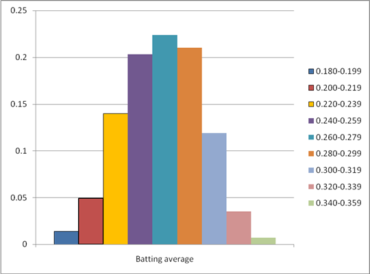
To construct: A relative frequency histogram for National League.
Explanation of Solution
Given information:The following frequency distribution presents the batting averages of Major League Baseball players in both the American League and the National League who had 300 or more plate appearances during a recent season.
| Batting average | American LeagueFrequency | National LeagueFrequency |
| 0.180-0.199 | 2 | 2 |
| 0.200-0.219 | 7 | 7 |
| 0.220-0.239 | 21 | 20 |
| 0.240-0.259 | 30 | 29 |
| 0.260-0.279 | 26 | 32 |
| 0.280-0.299 | 21 | 30 |
| 0.300-0.319 | 12 | 17 |
| 0.320-0.339 | 5 | 5 |
| 0.340-0.359 | 0 | 1 |
Definition used: Histograms based on relative frequency distributions are called relative frequency histogram.
Solution:
| Batting average | NationalLeagueRelative frequency |
| 0.180-0.199 | 0.014 |
| 0.200-0.219 | 0.049 |
| 0.220-0.239 | 0.140 |
| 0.240-0.259 | 0.203 |
| 0.260-0.279 | 0.224 |
| 0.280-0.299 | 0.210 |
| 0.300-0.319 | 0.119 |
| 0.320-0.339 | 0.035 |
| 0.340-0.359 | 0.007 |
The relative frequency histogram for the given data is given by

g.
To find: The percentage of American League players who had batting averages of 0.300 or more.
Answer to Problem 28E
The percentage of American League players who had batting averages of 0.300 or more is 13.7%.
Explanation of Solution
Given information:The following frequency distribution presents the batting averages of Major League Baseball players in both the American League and the National League who had 300 or more plate appearances during a recent season.
| Batting average | American LeagueFrequency | National LeagueFrequency |
| 0.180-0.199 | 2 | 2 |
| 0.200-0.219 | 7 | 7 |
| 0.220-0.239 | 21 | 20 |
| 0.240-0.259 | 30 | 29 |
| 0.260-0.279 | 26 | 32 |
| 0.280-0.299 | 21 | 30 |
| 0.300-0.319 | 12 | 17 |
| 0.320-0.339 | 5 | 5 |
| 0.340-0.359 | 0 | 1 |
Calculation:
The relative frequency for American League is given by
| Batting average | American LeagueRelative frequency |
| 0.180-0.199 | 0.016 |
| 0.200-0.219 | 0.056 |
| 0.220-0.239 | 0.169 |
| 0.240-0.259 | 0.242 |
| 0.260-0.279 | 0.210 |
| 0.280-0.299 | 0.169 |
| 0.300-0.319 | 0.097 |
| 0.320-0.339 | 0.040 |
| 0.340-0.359 | 0.000 |
From the above data, the relative frequencies of batting averages of 0.300 or more are 0.097, 0.040 and 0.000
The sum of all the above relative frequencies is
Then, its percentage is 13.7%
Hence, the percentage of American League players who had batting averages of 0.300 or more is 13.7%.
h.
To find: The percentage of National League players who had batting averages of 0.300 or more.
Answer to Problem 28E
The percentage of National League players who had batting averages of 0.300 or more is 16.1%.
Explanation of Solution
Given information:The following frequency distribution presents the batting averages of Major League Baseball players in both the American League and the National League who had 300 or more plate appearances during a recent season.
| Batting average | American LeagueFrequency | National LeagueFrequency |
| 0.180-0.199 | 2 | 2 |
| 0.200-0.219 | 7 | 7 |
| 0.220-0.239 | 21 | 20 |
| 0.240-0.259 | 30 | 29 |
| 0.260-0.279 | 26 | 32 |
| 0.280-0.299 | 21 | 30 |
| 0.300-0.319 | 12 | 17 |
| 0.320-0.339 | 5 | 5 |
| 0.340-0.359 | 0 | 1 |
Calculation:
The relative frequency for National League is given by
| Batting average | NationalLeagueRelative frequency |
| 0.180-0.199 | 0.014 |
| 0.200-0.219 | 0.049 |
| 0.220-0.239 | 0.140 |
| 0.240-0.259 | 0.203 |
| 0.260-0.279 | 0.224 |
| 0.280-0.299 | 0.210 |
| 0.300-0.319 | 0.119 |
| 0.320-0.339 | 0.035 |
| 0.340-0.359 | 0.007 |
From the above data, the relative frequencies of batting averages of 0.300 or more are 0.119, 0.035 and 0.007.
The sum of all the above relative frequencies is
Then, its percentage is 16.1%
Hence, the percentage of National League players who had batting averages of 0.300 or more is 16.1%.
i.
To find: The percentage of players who had batting averages less than 0.220.
Answer to Problem 28E
The batting averages tend to be a bit higher in the National League.
Explanation of Solution
Given information:The following frequency distribution presents the batting averages of Major League Baseball players in both the American League and the National League who had 300 or more plate appearances during a recent season.
| Batting average | American LeagueFrequency | National LeagueFrequency |
| 0.180-0.199 | 2 | 7 |
| 0.200-0.219 | 7 | 7 |
| 0.220-0.239 | 21 | 20 |
| 0.240-0.259 | 30 | 29 |
| 0.260-0.279 | 26 | 32 |
| 0.280-0.299 | 21 | 30 |
| 0.300-0.319 | 12 | 17 |
| 0.320-0.339 | 5 | 5 |
| 0.340-0.359 | 0 | 1 |
Solution:
The relative frequency histogram for American League is given by
The relative frequency histogram for the National League is given by
From the above two histograms, we can see that the relative frequency for National league is bit higher than the National League.
Hence, the batting averages tend to be a bit higher in the National League.
Want to see more full solutions like this?
Chapter 2 Solutions
Connect Hosted by ALEKS Online Access for Elementary Statistics
Additional Math Textbook Solutions
Precalculus: A Unit Circle Approach (3rd Edition)
College Algebra (Collegiate Math)
Intermediate Algebra (13th Edition)
Introductory Statistics
Basic College Mathematics


- 2PM Tue Mar 4 7 Dashboard Calendar To Do Notifications Inbox File Details a 25/SP-CIT-105-02 Statics for Technicians Q-7 Determine the resultant of the load system shown. Locate where the resultant intersects grade with respect to point A at the base of the structure. 40 N/m 2 m 1.5 m 50 N 100 N/m Fig.- Problem-7 4 m Gradearrow_forwardNsjsjsjarrow_forwardA smallish urn contains 16 small plastic bunnies - 9 of which are pink and 7 of which are white. 10 bunnies are drawn from the urn at random with replacement, and X is the number of pink bunnies that are drawn. (a) P(X=6)[Select] (b) P(X>7) ≈ [Select]arrow_forward
- A smallish urn contains 25 small plastic bunnies - 7 of which are pink and 18 of which are white. 10 bunnies are drawn from the urn at random with replacement, and X is the number of pink bunnies that are drawn. (a) P(X = 5)=[Select] (b) P(X<6) [Select]arrow_forwardElementary StatisticsBase on the same given data uploaded in module 4, will you conclude that the number of bathroom of houses is a significant factor for house sellprice? I your answer is affirmative, you need to explain how the number of bathroom influences the house price, using a post hoc procedure. (Please treat number of bathrooms as a categorical variable in this analysis)Base on the same given data, conduct an analysis for the variable sellprice to see if sale price is influenced by living area. Summarize your finding including all regular steps (learned in this module) for your method. Also, will you conclude that larger house corresponding to higher price (justify)?Each question need to include a spss or sas output. Instructions: You have to use SAS or SPSS to perform appropriate procedure: ANOVA or Regression based on the project data (provided in the module 4) and research question in the project file. Attach the computer output of all key steps (number) quoted in…arrow_forwardElementary StatsBase on the given data uploaded in module 4, change the variable sale price into two categories: abovethe mean price or not; and change the living area into two categories: above the median living area ornot ( your two group should have close number of houses in each group). Using the resulting variables,will you conclude that larger house corresponding to higher price?Note: Need computer output, Ho and Ha, P and decision. If p is small, you need to explain what type ofdependency (association) we have using an appropriate pair of percentages. Please include how to use the data in SPSS and interpretation of data.arrow_forward
- An environmental research team is studying the daily rainfall (in millimeters) in a region over 100 days. The data is grouped into the following histogram bins: Rainfall Range (mm) Frequency 0-9.9 15 10 19.9 25 20-29.9 30 30-39.9 20 ||40-49.9 10 a) If a random day is selected, what is the probability that the rainfall was at least 20 mm but less than 40 mm? b) Estimate the mean daily rainfall, assuming the rainfall in each bin is uniformly distributed and the midpoint of each bin represents the average rainfall for that range. c) Construct the cumulative frequency distribution and determine the rainfall level below which 75% of the days fall. d) Calculate the estimated variance and standard deviation of the daily rainfall based on the histogram data.arrow_forwardAn electronics company manufactures batches of n circuit boards. Before a batch is approved for shipment, m boards are randomly selected from the batch and tested. The batch is rejected if more than d boards in the sample are found to be faulty. a) A batch actually contains six faulty circuit boards. Find the probability that the batch is rejected when n = 20, m = 5, and d = 1. b) A batch actually contains nine faulty circuit boards. Find the probability that the batch is rejected when n = 30, m = 10, and d = 1.arrow_forwardTwenty-eight applicants interested in working for the Food Stamp program took an examination designed to measure their aptitude for social work. A stem-and-leaf plot of the 28 scores appears below, where the first column is the count per branch, the second column is the stem value, and the remaining digits are the leaves. a) List all the values. Count 1 Stems Leaves 4 6 1 4 6 567 9 3688 026799 9 8 145667788 7 9 1234788 b) Calculate the first quartile (Q1) and the third Quartile (Q3). c) Calculate the interquartile range. d) Construct a boxplot for this data.arrow_forward
- Pam, Rob and Sam get a cake that is one-third chocolate, one-third vanilla, and one-third strawberry as shown below. They wish to fairly divide the cake using the lone chooser method. Pam likes strawberry twice as much as chocolate or vanilla. Rob only likes chocolate. Sam, the chooser, likes vanilla and strawberry twice as much as chocolate. In the first division, Pam cuts the strawberry piece off and lets Rob choose his favorite piece. Based on that, Rob chooses the chocolate and vanilla parts. Note: All cuts made to the cake shown below are vertical.Which is a second division that Rob would make of his share of the cake?arrow_forwardThree players (one divider and two choosers) are going to divide a cake fairly using the lone divider method. The divider cuts the cake into three slices (s1, s2, and s3). If the choosers' declarations are Chooser 1: {s1 , s2} and Chooser 2: {s2 , s3}. Using the lone-divider method, how many different fair divisions of this cake are possible?arrow_forwardTheorem 2.6 (The Minkowski inequality) Let p≥1. Suppose that X and Y are random variables, such that E|X|P <∞ and E|Y P <00. Then X+YpX+Yparrow_forward
 Big Ideas Math A Bridge To Success Algebra 1: Stu...AlgebraISBN:9781680331141Author:HOUGHTON MIFFLIN HARCOURTPublisher:Houghton Mifflin Harcourt
 Holt Mcdougal Larson Pre-algebra: Student Edition...AlgebraISBN:9780547587776Author:HOLT MCDOUGALPublisher:HOLT MCDOUGAL
 Glencoe Algebra 1, Student Edition, 9780079039897...AlgebraISBN:9780079039897Author:CarterPublisher:McGraw Hill