Concept explainers
Videos
a.
Construct the percent frequency distribution for each degree.
a.
Answer to Problem 9E
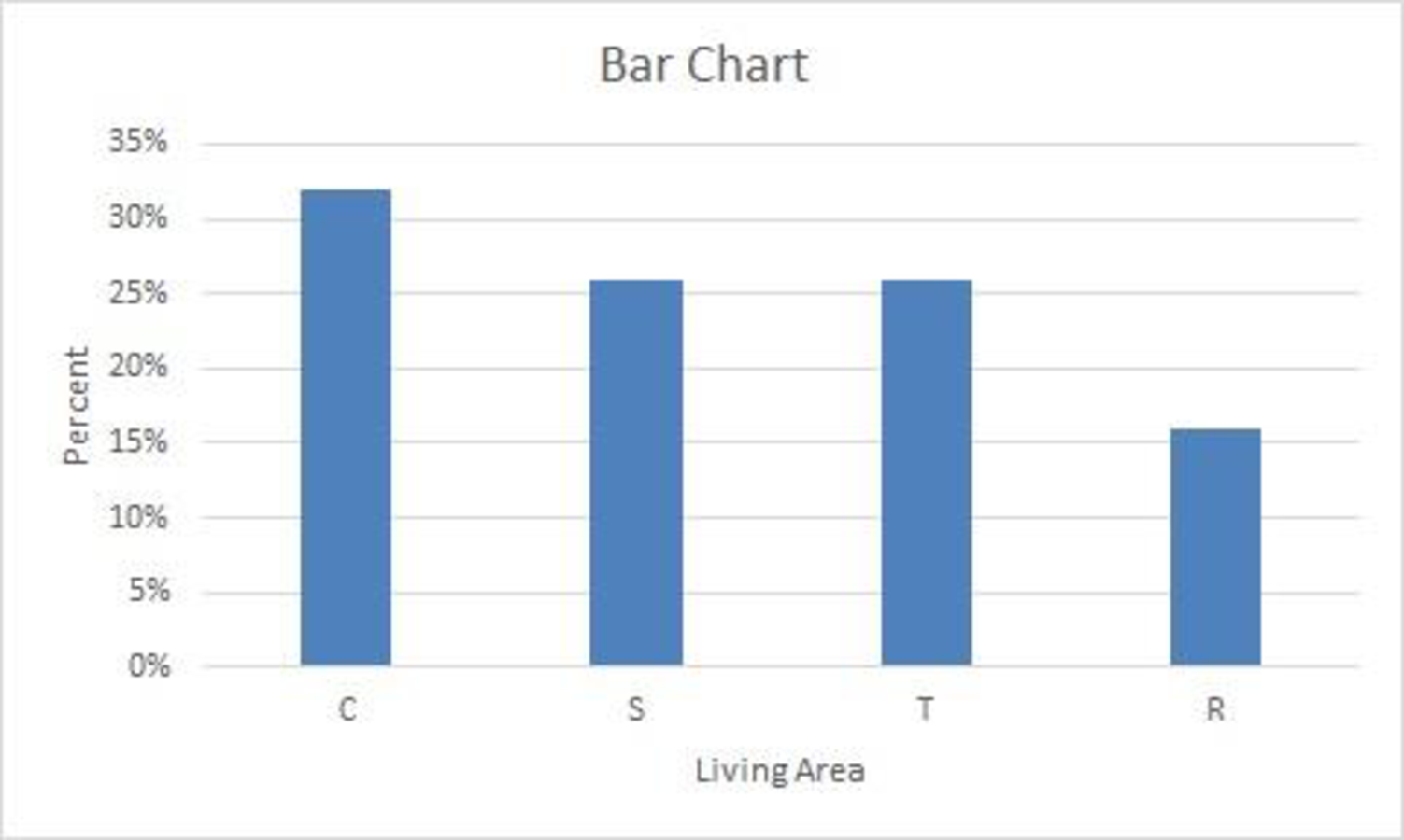
The percent frequency distributions for where the adults live now are given below:
| Responses | Percent frequency |
| C | 32% |
| S | 26% |
| T | 26% |
| R | 16% |
| Total | 100% |
The percent frequency distributions for ideal community are given below:
| Responses | Percent frequency |
| C | 24% |
| S | 25% |
| T | 30% |
| R | 21% |
| Total | 100% |
Explanation of Solution
Calculation:
The data represent 46% of adults from Country U who would live in a different type of community than the one where they are living now. A sample of 2,260 adults is surveyed. The response options are City(C), Suburb(S), Small Town(T), or Rural(R).
For living now:
Frequency:
The frequencies are calculated using the tally marks. Here, the number of times each class repeats is the frequency of that particular class.
Here, “C (city)” is the response data, which is repeated 32 times in the data set and thus, 32 is the frequency for the response “C (city)”.
Similarly, the frequencies of the remaining responses are as follows:
| Responses | Tally | Frequency |
| C | 32 | |
| S | 26 | |
| T | 26 | |
| R | 16 | |
| Total | 100 |
Relative frequency:
The general formula for relative frequency is given below:
Therefore, the following value is obtained:
Similarly, the relative frequencies for the remaining responses of a class are obtained below:
| Responses | Frequency | Relative frequency |
| C | 32 | 0.32 |
| S | 26 | |
| T | 26 | |
| R | 16 | |
| Total | 100 | 1.00 |
Percentage frequency distribution:
The general formula for percent frequency is given below:
Therefore, the following value is obtained:
The percent frequencies for the remaining responses for living now are obtained below:
| Responses | Relative frequency | Percent frequency |
| C | 0.32 | 32% |
| S | 0.26 | |
| T | 0.26 | |
| R | 0.16 | |
| Total | 1.00 | 100 |
For ideal community:
Here, “C (city)” is the response data, which is repeated 24 times in the data set and thus, 24 is the frequency for the response “C (city)”.
Similarly, the frequencies of the remaining types of department fields are given below:
| Responses | Tally | Frequency |
| C | 24 | |
| S | 25 | |
| T | 30 | |
| R | 21 | |
| Total | 100 |
Relative frequency:
Similarly, the relative frequencies for the remaining responses are obtained as follows:
| Responses | Frequency | Relative frequency |
| C | 24 | 0.24 |
| S | 25 | |
| T | 30 | |
| R | 21 | |
| Total | 100 | 1.00 |
Percentage frequency distribution:
The percent frequencies for the remaining responses for ideal community are obtained as follows:
| Responses | Relative frequency | Percent frequency |
| C | 0.24 | 24% |
| S | 0.25 | |
| T | 0.30 | |
| R | 0.21 | |
| Total | 1.00 | 100 |
b.
Construct the bar chart for each question.
b.
Answer to Problem 9E
Output obtained from Excel for the response of the first question is given below:
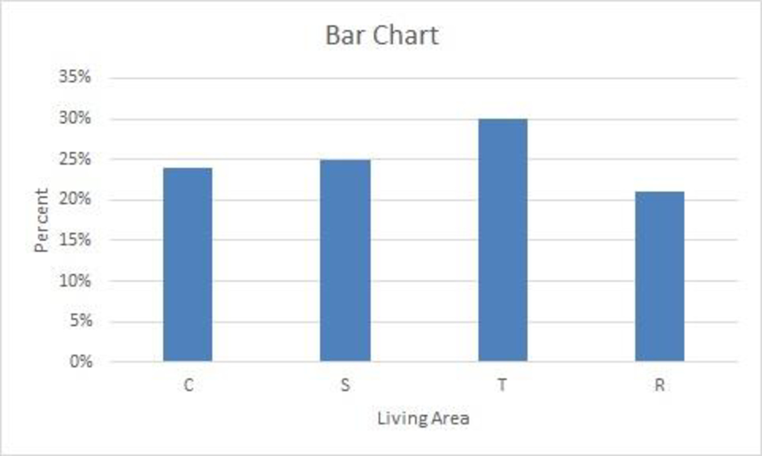
Output obtained from Excel for the response of the second question is given below:
Explanation of Solution
Calculation:
For living now:
Software procedure:
Step-by-step procedure to draw the bar chart for the first question using Excel:
- In Excel sheet, enter Living now in one column and Frequency in another column.
- Select the data and then choose Insert > Insert Column Bar Charts.
- Select Clustered Column Under More Column Charts.
- For ideal community:
Software procedure:
Step-by-step procedure to draw the bar chart for ideal community using Excel:
- In Excel sheet, enter Ideal community in one column and Frequency in another column.
- Select the data and then choose Insert > Insert Column Bar Charts.
- Select Clustered Column Under More Column Charts.
c.
Find the community in which most of the adults are living now.
c.
Answer to Problem 9E
Most of the adults are now living in a city.
Explanation of Solution
For living now, the percentage for city is 32%, which is high when compared to the other communities.
Thus, most of the adults are now living in a city.
d.
Identify the community that most of the adults consider as the ideal community.
d.
Answer to Problem 9E
Most of the adults consider the ideal community as a small town.
Explanation of Solution
For ideal community, the percentage for small town is 30%, which is high when compared to the other communities.
Thus, most of the adults consider the ideal community as a small town.
e.
Identify the changes in living areas that one would expect to see if people moved from where they currently live to their ideal community.
e.
Explanation of Solution
Calculation:
In order to obtain the changes in living areas when people moved from where they currently live to their ideal community, one would expect to find the difference between the two.
Therefore, the value is obtained as follows:
The differences between the living now and the ideal community are tabulated as follows:
| Responses | Living now | Ideal community | Difference |
| C | 32% | 24% | –8% |
| S | 26% | 25% | –1% |
| T | 26% | 30% | +4% |
| R | 16% | 21% | +5% |
From the table, it is observed that the living area “city” has the largest decrease in percentage from living now to ideal community. For suburb, living is steady. For small towns and rural areas, the percentage of living increases.
Want to see more full solutions like this?
Chapter 2 Solutions
Modern Business Statistics with Microsoft Excel (MindTap Course List)


- Suppose a random sample of 459 married couples found that 307 had two or more personality preferences in common. In another random sample of 471 married couples, it was found that only 31 had no preferences in common. Let p1 be the population proportion of all married couples who have two or more personality preferences in common. Let p2 be the population proportion of all married couples who have no personality preferences in common. Find a95% confidence interval for . Round your answer to three decimal places.arrow_forwardA history teacher interviewed a random sample of 80 students about their preferences in learning activities outside of school and whether they are considering watching a historical movie at the cinema. 69 answered that they would like to go to the cinema. Let p represent the proportion of students who want to watch a historical movie. Determine the maximal margin of error. Use α = 0.05. Round your answer to three decimal places. arrow_forwardA random sample of medical files is used to estimate the proportion p of all people who have blood type B. If you have no preliminary estimate for p, how many medical files should you include in a random sample in order to be 99% sure that the point estimate will be within a distance of 0.07 from p? Round your answer to the next higher whole number.arrow_forward
- A clinical study is designed to assess the average length of hospital stay of patients who underwent surgery. A preliminary study of a random sample of 70 surgery patients’ records showed that the standard deviation of the lengths of stay of all surgery patients is 7.5 days. How large should a sample to estimate the desired mean to within 1 day at 95% confidence? Round your answer to the whole number.arrow_forwardA clinical study is designed to assess the average length of hospital stay of patients who underwent surgery. A preliminary study of a random sample of 70 surgery patients’ records showed that the standard deviation of the lengths of stay of all surgery patients is 7.5 days. How large should a sample to estimate the desired mean to within 1 day at 95% confidence? Round your answer to the whole number.arrow_forwardIn the experiment a sample of subjects is drawn of people who have an elbow surgery. Each of the people included in the sample was interviewed about their health status and measurements were taken before and after surgery. Are the measurements before and after the operation independent or dependent samples?arrow_forward
- iid 1. The CLT provides an approximate sampling distribution for the arithmetic average Ỹ of a random sample Y₁, . . ., Yn f(y). The parameters of the approximate sampling distribution depend on the mean and variance of the underlying random variables (i.e., the population mean and variance). The approximation can be written to emphasize this, using the expec- tation and variance of one of the random variables in the sample instead of the parameters μ, 02: YNEY, · (1 (EY,, varyi n For the following population distributions f, write the approximate distribution of the sample mean. (a) Exponential with rate ẞ: f(y) = ß exp{−ßy} 1 (b) Chi-square with degrees of freedom: f(y) = ( 4 ) 2 y = exp { — ½/ } г( (c) Poisson with rate λ: P(Y = y) = exp(-\} > y! y²arrow_forward2. Let Y₁,……., Y be a random sample with common mean μ and common variance σ². Use the CLT to write an expression approximating the CDF P(Ỹ ≤ x) in terms of µ, σ² and n, and the standard normal CDF Fz(·).arrow_forwardmatharrow_forward
- Compute the median of the following data. 32, 41, 36, 42, 29, 30, 40, 22, 25, 37arrow_forwardTask Description: Read the following case study and answer the questions that follow. Ella is a 9-year-old third-grade student in an inclusive classroom. She has been diagnosed with Emotional and Behavioural Disorder (EBD). She has been struggling academically and socially due to challenges related to self-regulation, impulsivity, and emotional outbursts. Ella's behaviour includes frequent tantrums, defiance toward authority figures, and difficulty forming positive relationships with peers. Despite her challenges, Ella shows an interest in art and creative activities and demonstrates strong verbal skills when calm. Describe 2 strategies that could be implemented that could help Ella regulate her emotions in class (4 marks) Explain 2 strategies that could improve Ella’s social skills (4 marks) Identify 2 accommodations that could be implemented to support Ella academic progress and provide a rationale for your recommendation.(6 marks) Provide a detailed explanation of 2 ways…arrow_forwardQuestion 2: When John started his first job, his first end-of-year salary was $82,500. In the following years, he received salary raises as shown in the following table. Fill the Table: Fill the following table showing his end-of-year salary for each year. I have already provided the end-of-year salaries for the first three years. Calculate the end-of-year salaries for the remaining years using Excel. (If you Excel answer for the top 3 cells is not the same as the one in the following table, your formula / approach is incorrect) (2 points) Geometric Mean of Salary Raises: Calculate the geometric mean of the salary raises using the percentage figures provided in the second column named “% Raise”. (The geometric mean for this calculation should be nearly identical to the arithmetic mean. If your answer deviates significantly from the mean, it's likely incorrect. 2 points) Starting salary % Raise Raise Salary after raise 75000 10% 7500 82500 82500 4% 3300…arrow_forward
 Holt Mcdougal Larson Pre-algebra: Student Edition...AlgebraISBN:9780547587776Author:HOLT MCDOUGALPublisher:HOLT MCDOUGAL
 Big Ideas Math A Bridge To Success Algebra 1: Stu...AlgebraISBN:9781680331141Author:HOUGHTON MIFFLIN HARCOURTPublisher:Houghton Mifflin Harcourt
 Glencoe Algebra 1, Student Edition, 9780079039897...AlgebraISBN:9780079039897Author:CarterPublisher:McGraw Hill
 College Algebra (MindTap Course List)AlgebraISBN:9781305652231Author:R. David Gustafson, Jeff HughesPublisher:Cengage Learning