Concept explainers
Videos
Decimal Data: Batting Averages The following data represent baseball batting averages for a random sample of National League players neat the end of the baseball season. the data are from the baseball statistics section of the Denver Post.
| 0.194 | 0.258 | 0.190 | 0.291 | 0.158 | 0.295 | 0.261 | 0.250 | 0.181 |
| 0.125 | 0.107 | 0.260 | 0.309 | 0.309 | 0.276 | 0.287 | 0.317 | 0.252 |
| 0.215 | 0.250 | 0.246 | 0.260 | 0.265 | 0.182 | 0.113 | 0.200 |
(a) Multiply each data value by 1000 to “clear” the decimals.
(b) Use the standard procedares of this section to make a frequency table and histogram with your whole-number data. Use five classes.
(c) Divide class limits, class boundaries, and class midpoints by 1000 to get back to your original dat.
(a)
To find: The decimal data that are multiply with 1000 for each value in the data..
Answer to Problem 22P
Solution: The data multiply with 1000 for each value in the data is as follows:
| Data | Data*100 | Data | Data*100 |
| 0.194 | 194 | 0.309 | 309 |
| 0.258 | 258 | 0.276 | 276 |
| 0.19 | 190 | 0.287 | 287 |
| 0.291 | 291 | 0.317 | 317 |
| 0.158 | 158 | 0.252 | 252 |
| 0.295 | 295 | 0.215 | 215 |
| 0.261 | 261 | 0.25 | 250 |
| 0.25 | 250 | 0.246 | 246 |
| 0.181 | 181 | 0.26 | 260 |
| 0.125 | 125 | 0.265 | 265 |
| 0.107 | 107 | 0.182 | 182 |
| 0.26 | 260 | 0.113 | 113 |
| 0.309 | 309 | 0.2 | 200 |
Explanation of Solution
Calculation: The data represent baseball batting averages for a random sample of National League players near the end of the baseball season and there are 26 values in the data set. To find the whole number data by multiplying 1000 is obtained as follows:
| Data | Data*100 | Data | Data*100 |
| 0.194 | 0.309 | 309 | |
| 0.258 | 0.276 | 276 | |
| 0.19 | 0.287 | 287 | |
| 0.291 | 291 | 0.317 | 317 |
| 0.158 | 158 | 0.252 | 252 |
| 0.295 | 295 | 0.215 | 215 |
| 0.261 | 261 | 0.25 | 250 |
| 0.25 | 250 | 0.246 | 246 |
| 0.181 | 181 | 0.26 | 260 |
| 0.125 | 125 | 0.265 | 265 |
| 0.107 | 107 | 0.182 | 182 |
| 0.26 | 260 | 0.113 | 113 |
| 0.309 | 309 | 0.2 | 200 |
Interpretation: Hence, the data multiply with 1000 is as follows:
| Data | Data*100 | Data | Data*100 |
| 0.194 | 194 | 0.309 | 309 |
| 0.258 | 258 | 0.276 | 276 |
| 0.19 | 190 | 0.287 | 287 |
| 0.291 | 291 | 0.317 | 317 |
| 0.158 | 158 | 0.252 | 252 |
| 0.295 | 295 | 0.215 | 215 |
| 0.261 | 261 | 0.25 | 250 |
| 0.25 | 250 | 0.246 | 246 |
| 0.181 | 181 | 0.26 | 260 |
| 0.125 | 125 | 0.265 | 265 |
| 0.107 | 107 | 0.182 | 182 |
| 0.26 | 260 | 0.113 | 113 |
| 0.309 | 309 | 0.2 | 200 |
(b)
To find: The standard frequency table for the data set..
Answer to Problem 22P
Solution: The complete frequency table is as:
| Class limits | Class boundaries | Midpoints | Freq | Relative freq | Cumulative freq |
| 46-85 | 45.5-85.5 | 65.5 | 4 | 0.12 | 4 |
| 86-125 | 85.5-125.5 | 105.5 | 5 | 0.16 | 9 |
| 126-165 | 125.5-165.5 | 145.5 | 10 | 0.31 | 19 |
| 166-205 | 165.5-205.5 | 185.5 | 5 | 0.16 | 24 |
| 206-245 | 205.5-245.5 | 225.5 | 5 | 0.16 | 29 |
| 246-285 | 245.5-285.5 | 265.5 | 3 | 0.09 | 32 |
Explanation of Solution
Calculation: To find the class width for the whole data of 26 values, it is observed that largest value of the data set is 317 and the smallest value is 107 in the data. Using 5 classes, the class width calculated in the following way:
The value is round up to the nearest whole number. Hence, the class width of the data set is 43. The class width for the data is 43 and the lowest data value (107) will be the lower class limit of the first class. Because the class width is 43, it must add 43 to the lowest class limit in the first class to find the lowest class limit in the second class. There are 5 desired classes. Hence, the class limits are 107–149, 150–192, 193–235, 236–278, and 279–321. Now, to find the class boundaries subtract 0.5 from lower limit of every class and add 0.5 to the upper limit of the every class interval. Hence, the class boundaries are 106.5–149.5, 149.5–192.5, 192.5–235.5, 235.5-278.5, and 278.5-321.5.
Next to find the midpoint of the class is calculated by using formula,
Midpoint of first class is calculated as:
The frequencies for respective classes are 3, 4, 3, 10, and 6.
Relative frequency is calculated by using the formula
The frequency for first class is 3 and total frequencies are 26 so the relative frequency is
The calculated frequency table is as follows:
| Class limits | Class boundaries | Midpoints | freq | relative freq |
| 107-149 | 106.5-149.5 | 128 | 3 | 0.12 |
| 150-192 | 149.5-192.5 | 171 | 4 | 0.15 |
| 193-235 | 192.5-235.5 | 214 | 3 | 0.12 |
| 236-278 | 235.5-278.5 | 257 | 10 | 0.38 |
| 279-321 | 278.5-321.5 | 300 | 6 | 0.23 |
Graph: To construct the histogram by using the MINITAB, the steps are as follows:
Step 1: Enter the class boundaries in C1 and frequency in C2.
Step 2: Go to Graph > Histogram > Simple.
Step 3: Enter C1 in Graph variable then go to Data options > Frequency > C2.
Step 4: Click on OK.
The obtained histogram is
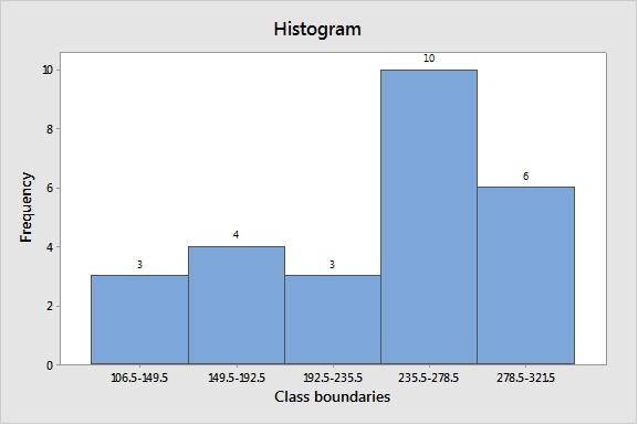
Interpretation: Hence, the complete frequency table is as follows:
| Class limits | Class boundaries | Midpoints | Freq | Relative freq |
| 107-149 | 106.5-149.5 | 128 | 3 | 0.12 |
| 150-192 | 149.5-192.5 | 171 | 4 | 0.15 |
| 193-235 | 192.5-235.5 | 214 | 3 | 0.12 |
| 236-278 | 235.5-278.5 | 257 | 10 | 0.38 |
| 279-321 | 278.5-321.5 | 300 | 6 | 0.23 |
(c)
To find: The class limits, class boundaries, and midpoints in the frequency table by dividing 1000..
Answer to Problem 22P
Solution: The frequency table of original data is as follows:
| Class limits | Class boundaries | Midpoints | |
| 0.107-0.149 | 0.1065-0.1495 | 0.128 | |
| 0.149-0.192 | 0.1495-0.1925 | 0.171 | |
| 0.193-0.235 | 0.1925-0.2355 | 0.214 | |
| 0.236-0.278 | 0.2355-0.2785 | 0.257 | |
| 0.279-0.321 | 0.2785-0.3215 | 0.3 | |
Explanation of Solution
Calculation: The frequency table for whole number is obtained in above part. It is the data that multiply each value by 1000 to ‘clear’ decimals from the data. The frequency table for whole number is as follows:
| Class limits | Class boundaries | Midpoints | Freq | Relative freq |
| 107–149 | 106.5–149.5 | 128 | 3 | 0.12 |
| 150–192 | 149.5–192.5 | 171 | 4 | 0.15 |
| 193–235 | 192.5–235.5 | 214 | 3 | 0.12 |
| 236–278 | 235.5–278.5 | 257 | 10 | 0.38 |
| 279–321 | 278.5–321.5 | 300 | 6 | 0.23 |
To find the decimal or original data, divide the class limits, class boundaries, and midpoints by 1000. The calculation as follows:
| Class limits | Class boundaries | Midpoints | |
| 0.107–0.149 | 0.1065–0.1495 | 0.128 | |
| 0.149–0.192 | 0.1495–0.1925 | 0.171 | |
| 0.193–0.235 | 0.1925–0.2355 | 0.214 | |
| 0.236–0.278 | 0.2355–0.2785 | 0.257 | |
| 0.279–0.321 | 0.2785–0.3215 | 0.3 | |
Interpretation: Hence, the data divide by 1000 is as follows:
| Class limits | Class boundaries | Midpoints | |
| 0.107–0.149 | 0.1065–0.1495 | 0.128 | |
| 0.149–0.192 | 0.1495–0.1925 | 0.171 | |
| 0.193–0.235 | 0.1925–0.2355 | 0.214 | |
| 0.236–0.278 | 0.2355–0.2785 | 0.257 | |
| 0.279–0.321 | 0.2785–0.3215 | 0.300 | |
Want to see more full solutions like this?
Chapter 2 Solutions
Understanding Basic Statistics


- solve the question based on hw 1, 1.41arrow_forwardT1.4: Let ẞ(G) be the minimum size of a vertex cover, a(G) be the maximum size of an independent set and m(G) = |E(G)|. (i) Prove that if G is triangle free (no induced K3) then m(G) ≤ a(G)B(G). Hints - The neighborhood of a vertex in a triangle free graph must be independent; all edges have at least one end in a vertex cover. (ii) Show that all graphs of order n ≥ 3 and size m> [n2/4] contain a triangle. Hints - you may need to use either elementary calculus or the arithmetic-geometric mean inequality.arrow_forwardWe consider the one-period model studied in class as an example. Namely, we assumethat the current stock price is S0 = 10. At time T, the stock has either moved up toSt = 12 (with probability p = 0.6) or down towards St = 8 (with probability 1−p = 0.4).We consider a call option on this stock with maturity T and strike price K = 10. Theinterest rate on the money market is zero.As in class, we assume that you, as a customer, are willing to buy the call option on100 shares of stock for $120. The investor, who sold you the option, can adopt one of thefollowing strategies: Strategy 1: (seen in class) Buy 50 shares of stock and borrow $380. Strategy 2: Buy 55 shares of stock and borrow $430. Strategy 3: Buy 60 shares of stock and borrow $480. Strategy 4: Buy 40 shares of stock and borrow $280.(a) For each of strategies 2-4, describe the value of the investor’s portfolio at time 0,and at time T for each possible movement of the stock.(b) For each of strategies 2-4, does the investor have…arrow_forward
- Negate the following compound statement using De Morgans's laws.arrow_forwardNegate the following compound statement using De Morgans's laws.arrow_forwardQuestion 6: Negate the following compound statements, using De Morgan's laws. A) If Alberta was under water entirely then there should be no fossil of mammals.arrow_forward
- Negate the following compound statement using De Morgans's laws.arrow_forwardCharacterize (with proof) all connected graphs that contain no even cycles in terms oftheir blocks.arrow_forwardLet G be a connected graph that does not have P4 or C3 as an induced subgraph (i.e.,G is P4, C3 free). Prove that G is a complete bipartite grapharrow_forward
 Big Ideas Math A Bridge To Success Algebra 1: Stu...AlgebraISBN:9781680331141Author:HOUGHTON MIFFLIN HARCOURTPublisher:Houghton Mifflin Harcourt
 Glencoe Algebra 1, Student Edition, 9780079039897...AlgebraISBN:9780079039897Author:CarterPublisher:McGraw Hill
 Holt Mcdougal Larson Pre-algebra: Student Edition...AlgebraISBN:9780547587776Author:HOLT MCDOUGALPublisher:HOLT MCDOUGAL