Videos
a.
Calculate the class width for the data on count of three-syllable words in advertising copy of magazine advertisements.
a.
Answer to Problem 20P
The class width is calculated as 6.
Explanation of Solution
Calculation:
From the given data set, the largest data point is 43 and the smallest data point is 0.
Class Width:
The class width is calculated as follows:
b.
Create a table for frequency distribution with class limits, class boundaries, midpoints, frequencies, relative frequencies, and cumulative frequencies.
b.
Answer to Problem 20P
The class limits for a frequency table with 8 classes using class width 6 are 0-5, 6-11, 12-17, 18-23, 24-29, 30-35, 36-41, and 42-47.
Explanation of Solution
Class limits:
Class limits are the maximum and minimum values in the class interval
Class Boundaries:
A class boundary is the midpoint between the upper limit of one class and the lower limit of the next class where the upper limit of the preceding class interval and the lower limit of the next class interval will be equal. The upper class boundary is calculated by adding 0.5 to the upper class limit and the lower class boundary is calculated by subtracting 0.5 from the lower class limit.
Midpoint:
The midpoint is calculated as given below:
Frequency:
Frequency is the number of data points that fall under each class.
Cumulative frequency:
Cumulative frequency is calculated by adding each frequency to the sum of preceding frequencies.
Relative Frequency:
Relative frequency is the ratio of frequency by the total number of data values.
The class width is 6. Hence, the lower class limit for the second class 6 is calculated by adding 6 to 0. Following this pattern, all the lower class limits are established. Then, the upper class limits are calculated.
The frequency distribution table is given below:
| Class Limits | Class Boundaries | Midpoints | Frequency | Relative Frequency | Cumulative Frequency |
| 0-5 | 0.5-5.5 |
2.5 | 13 | 13 | |
| 6-11 | 5.5-11.5 | 8.5 | 15 | 28 (=15+13) | |
| 12-17 | 11.5-17.5 | 14.5 | 11 | 39 (=11+28) | |
| 18-23 | 17.5-23.5 | 20.5 | 3 | 42 (=3+39) | |
| 24-29 | 23.5-29.5 | 26.5 | 6 | 48 (=6+42) | |
| 30-35 | 29.5-35.5 | 32.5 | 4 | 52 (=4+48) | |
| 36-41 | 35.5-41.5 | 38.5 | 2 | 54 (=2+52) | |
| 42-47 | 41.5-47.5 | 44.5 | 1 | 55 (=1+54) |
c.
Create a histogram for the given data on count of three-syllable words in advertising copy of magazine advertisements.
c.
Answer to Problem 20P
The frequency histogram for the data on count of three-syllable words in advertising copy of magazine advertisements is shown below:

Explanation of Solution
Step-by-step procedure to draw the histogram using MINITAB software:
- Choose Graph > Bar Chart.
- From Bars represent, choose Values from a table.
- Under One column of values, choose Simple. Click OK.
- In Graph variables, enter the column of Frequency.
- In Categorical variables, enter the column of Three-syllable Words.
- Click OK.
Thus, the histogram for three-syllable word data is obtained.
d.
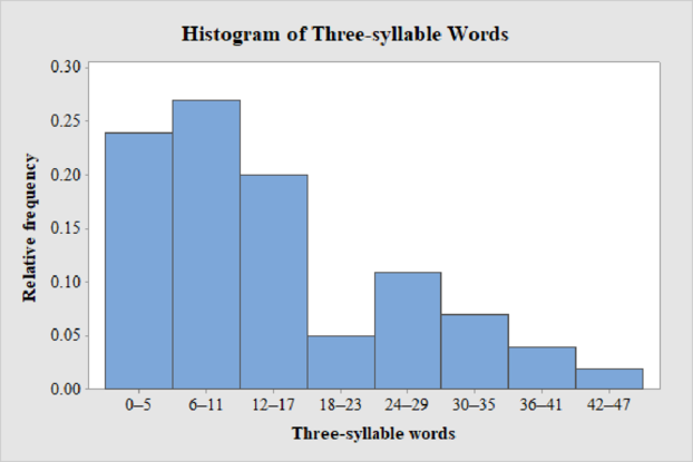
Construct a relative frequency histogram for the data on count of three-syllable words in advertising copy of magazine advertisements.
d.
Answer to Problem 20P
The relative frequency histogram for the data on count of three-syllable words in advertising copy of magazine advertisements is shown below:
Explanation of Solution
Step-by-step procedure to draw the histogram using MINITAB software:
- Choose Graph > Bar Chart.
- From Bars represent, choose Values from a table.
- Under One column of values, choose Simple. Click OK.
- In Graph variables, enter the column of Relative frequency.
- In Categorical variables, enter the column of Three-syllable Words.
- Click OK.
Thus, the relative frequency histogram for three-syllable word data is obtained.
e.
Identify the shape of distribution: uniform, mound shaped, symmetric, bimodal, skewed left, or skewed right.
e.
Explanation of Solution
From the histogram, the distribution of count of three-syllable words in advertising copy of magazine advertisements is skewed to the right.
f.
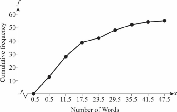
Create an ogive curve for the given data on count of three-syllable words in advertising copy of magazine advertisements.
f.
Answer to Problem 20P
An ogive curve for the count of three-syllable words in advertising copy of magazine advertisements is shown below:
Explanation of Solution
Step-by-step procedure to draw the Ogive curve:
- Draw X axis with data values ranging from -0.5 to 47.5.
- Label the X axis as Number of Words.
- Draw Y axis with data values Cumulative frequency ranging from.0 to 60.
- Label the Y axis as Cumulative frequency.
- Plot the cumulative frequencies
- Join the points and draw an ogive curve.
Thus, an ogive curve for three-syllable word data is obtained.
g.
Identify the characteristics about the count of three-syllable words in advertising copy of magazine advertisements using the graphs.
g.
Explanation of Solution
The data values of count of three-syllable words in advertising copy of magazine advertisements fall within 0 and 43.
The
The central value of the data is approximately 11.5.
From the histogram, it can be observed that the data is skewed to the right and there are no unusual observations in the data as not even one data point is far from the overall bulk of data.
Want to see more full solutions like this?
Chapter 2 Solutions
Bundle: Understandable Statistics, Loose-leaf Version, 12th + WebAssign Printed Access Card for Brase/Brase's Understandable Statistics: Concepts and Methods, 12th Edition, Single-Term


- A fitness trainer wants to estimate the effect of fitness activities on muscle mass for different weight categories of club members. They choose the most popular fitness classes at the gym: yoga, circuit training, and high-intensity interval training (HIIT). Suppose that the weights of club members are separated into three levels: under 155 pounds, 155 – 200 pounds, and over 200 pounds. Draw a flow chart showing the design of this experiment.arrow_forwardThe systolic blood pressure of individuals is thought to be related to both age and weight. Let the systolic blood pressure, age, and weight be represented by the variables x1, x2, and x3, respectively. Suppose that Minitab was used to generate the following descriptive statistics, correlations, and regression analysis for a random sample of 15 individuals. Descriptive Statistics Variable N Mean Median TrMean StDev SE Mean x 1 15 154.14 154.34 154.14 3.842 0.992000 x 2 15 59.69 60.19 59.69 1.462 0.377487 x 3 15 205.55 204.75 205.55 4.558 1.176871 Variable Minimum Maximum Q1 Q3 x 1 125 178 141.803 167.244 x 2 41 80 47.754 78.415 x 3 126 240 140.395 224.008 Correlations (Pearson) x 1 x 2 x 2 0.892 x 3 0.839 0.567 Regression Analysis The regression equation is x 1 = 0.883 + 1.257x2 + 0.871x3 Predictor Coef StDev T P Constant 0.883 0.635 1.39 0.095 x 2 1.257 0.635 1.98 0.036 x 3 0.871 0.419 2.08 0.030 S = 0.428 R-sq = 92.7 %…arrow_forwardAccording to health professionals, a person’s weight is expected to increase with age. To examine that statement, a nutritionist collected data from 11 random females from different age categories between the ages of 21 and 43. In the following table, x is the age of a person and y is the weight in pounds. x, age 21 24 27 29 31 33 35 38 40 42 43 y, weight in lb 121.4 122.3 130.3 131.7 133.3 134.6 136.7 138.4 140.3 142.0 145.1 Select the correct graph of the least-squares line on a scatter diagram.arrow_forward
- Let x be a random variable that represents the percentage of successful free throws a professional basketball player makes in a season. Let y be a random variable that represents the percentage of successful field goals a professional basketball player makes in a season. A random sample of n = 6 professional basketball players gave the following information. x 82 69 73 84 74 64 y 42 48 46 46 46 42 Verify that ∑x =446, ∑y =270, ∑x2 =33,442, ∑y2 =12,180, ∑xy =20,070, and r = 0, and find the critical value for a test using a 5% level of significance claiming that ρis not equal than zero. Round your answer to three decimal places.arrow_forwardLet x be a random variable that represents the percentage of successful free throws a professional basketball player makes in a season. Let y be a random variable that represents the percentage of successful field goals a professional basketball player makes in a season. A random sample of n = 6 professional basketball players gave the following information. x 75 72 75 81 74 81 y 46 39 42 47 49 50 Verify that Se ࣈ 3.591,a ࣈ –10.145, bࣈ0.729, and , and find the predicted percentage of successful field goals for a player with x= 88%successful free throws. Round your answer to the nearest tenth of a percentarrow_forwardAn editor wants to analyze if there is a significant difference in the ratings of books in four different genres. Random samples of book ratings were collected for four different genres. The editor recorded ratings in a 0 to 10 scale in the following table. Fiction Novel Biography Science&Technology 8.5 8.4 6.2 9.1 5.3 5.3 5.5 4.3 7.7 4.2 7.0 9.7 5.1 9.8 9.3 5.2 6.9 8.6 6.7 7.9 4.8 7.1 6.9 8.4 Shall we reject or not reject the claim that there are no differences among the population means of book ratings for the different genres? Use.arrow_forward
- Peggy conducted a study to identify the randomness of rainy days in fall. For 15 days, she recorded whether it rained that day or not. They denoted a rainy day with the letter R, a day without rain with the letter N. R N N R R N N R R N N R R R R Test the sequence for randomness. Use .arrow_forwardConsider the grades for the math and history exams for 10 students on a scale from 0 to 12 in the following table. Student Math History 1 4 8 2 5 9 3 7 9 4 12 10 5 10 8 6 8 5 7 9 6 8 9 6 9 11 9 10 7 10 Compute the Spearman correlation coefficient. Round your answer to three decimal places.arrow_forwardTo compare two elementary schools regarding teaching of reading skills, 12 sets of identical twins were used. In each case, one child was selected at random and sent to school A, and his or her twin was sent to school B. Near the end of fifth grade, an achievement test was given to each child. The results follow: Twin Pair 1 2 3 4 5 6 School A 169 157 115 99 119 113 School B 123 157 112 99 121 122 Twin Pair 7 8 9 10 11 12 School A 120 121 124 145 138 117 School B 153 90 124 140 142 102 Suppose a sign test for matched pairs with a 1% level of significance is used to test the hypothesis that the schools have the same effectiveness in teaching reading skills against the alternate hypothesis that the schools have different levels of effectiveness in teaching reading skills. Let p denote portion of positive signs when the scores of school B are subtracted from the corresponding scores of school…arrow_forward
- A horse trainer teaches horses to jump by using two methods of instruction. Horses being taught by method A have a lead horse that accompanies each jump. Horses being taught by method B have no lead horse. The table shows the number of training sessions required before each horse performed the jumps properly. Method A 25 23 39 29 37 20 Method B 41 21 46 42 24 44 Method A 45 35 27 31 34 49 Method B 26 43 47 32 40 Use a rank-sum test with a5% level of significance to test the claim that there is no difference between the training sessions distributions. If the value of the sample test statistic R, the rank-sum, is 150, calculate the P-value. Round your answer to four decimal places.arrow_forwardA data processing company has a training program for new salespeople. After completing the training program, each trainee is ranked by his or her instructor. After a year of sales, the same class of trainees is again ranked by a company supervisor according to net value of the contracts they have acquired for the company. The results for a random sample of 11 salespeople trained in the last year follow, where x is rank in training class and y is rank in sales after 1 year. Lower ranks mean higher standing in class and higher net sales. Person 1 2 3 4 5 6 x rank 8 11 2 4 5 3 y rank 7 10 1 3 2 4 Person 7 8 9 10 11 x rank 7 9 10 1 6 y rank 8 11 9 6 5 Using a 1% level of significance, test the claim that the relation between x and y is monotone (either increasing or decreasing). Verify that the Spearman rank correlation coefficient . This implies that the P-value lies between 0.002 and 0.01. State…arrow_forwardSand and clay studies were conducted at a site in California. Twelve consecutive depths, each about 15 cm deep, were studied and the following percentages of sand in the soil were recorded. 34.4 27.1 30.8 28.0 32.2 27.6 32.8 25.2 31.4 33.5 24.7 28.4 Converting this sequence of numbers to a sequence of symbols A and B, where A indicates a value above the median and B denotes a value below the median gives ABABABABAABB. Test the sequence for randomness about the median with a 5% level of significance. Verify that the number of runs is 10. What is the upper critical value c2? arrow_forward
 Holt Mcdougal Larson Pre-algebra: Student Edition...AlgebraISBN:9780547587776Author:HOLT MCDOUGALPublisher:HOLT MCDOUGAL
 Glencoe Algebra 1, Student Edition, 9780079039897...AlgebraISBN:9780079039897Author:CarterPublisher:McGraw Hill
 Big Ideas Math A Bridge To Success Algebra 1: Stu...AlgebraISBN:9781680331141Author:HOUGHTON MIFFLIN HARCOURTPublisher:Houghton Mifflin Harcourt
 Functions and Change: A Modeling Approach to Coll...AlgebraISBN:9781337111348Author:Bruce Crauder, Benny Evans, Alan NoellPublisher:Cengage Learning