
Concept explainers
Videos
(a)
To graph: The
(a)
Explanation of Solution
Graph: To draw the scatterplot for the provided data set, the below steps are followed in Minitab software.
Step 1: Open the “MEIS” file in Minitab software.
Step 2: Go to Graph
Step 3: Choose the option “Simple” and click “OK”.
Step 4: Select “Sales” as Y variables and “Dwellpermit” as X variables.
Step 5: Click “OK” twice.
The scatterplot is obtained as:
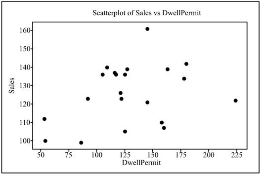
To explain: The relationship between the variables and the presence of the outliers.
Answer to Problem 144E
Solution: Though the relationship between the variables is very weak, but there is no outlier in the data set.
Explanation of Solution
(b)
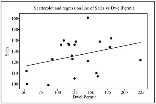
To find: The least-squares regression line for the data.
(b)
Answer to Problem 144E
Solution: The least-squares regression line is obtained as
Explanation of Solution
Calculation: To draw the regression line and obtain the sketch of the regression line, the below steps are followed in the Minitab software.
Step 1: Right click on the obtained graph in the part (a).
Step 2: Go to Add
Step 3: Click on “Linear” under the menu “Model Order” and tick the “Fit intercept”.
Step 4: Click on “OK” to obtain the regression line.
The obtained regression equation is
Graph: The below graph shows the regression line.

(c)
To explain: The slope of the obtained line.
(c)
Answer to Problem 144E
Solution: The slope can be interpreted as if there is an increase of 1unit of the variable, issued permit for dwelling then there is an increase of 0.1263 units in the value of the variable sales.
Explanation of Solution
(d)
To explain: The intercept of the line.
(d)
Answer to Problem 144E
Solution: The intercept can be interpreted as the value of the response variable when the value of the explanatory variable is zero. As the value of the response variable is 109.8 for the zero issued permits, it is appropriate to use the intercept for explaining the relationship between the variables.
Explanation of Solution
(e)
The sales for an index of 224 dwelling permits.
(e)
Answer to Problem 144E
Solution: The predicted value of the sales is 138.0912.
Explanation of Solution
The predicted value can be calculated as:
(f)
To find: The residual value for Canada.
(f)
Answer to Problem 144E
Solution: The obtained value of the residual is
Explanation of Solution
Calculation: The sale for the Canada is provided as 122. The residual value for the sales for Canada whose index of dwelling permits is 224 is calculated as:
(g)
The percentage of variability in sales is explained by dwelling permit.
(g)
Answer to Problem 144E
Solution: The explained percentage of variability in sales is 10.30%.
Explanation of Solution
Therefore, the proportion of variation that is explained by the explanatory variables of the model is 10.30%.
Want to see more full solutions like this?
Chapter 2 Solutions
Introduction to the Practice of Statistics


- Business discussarrow_forwardBusiness discussarrow_forwardI just need to know why this is wrong below: What is the test statistic W? W=5 (incorrect) and What is the p-value of this test? (p-value < 0.001-- incorrect) Use the Wilcoxon signed rank test to test the hypothesis that the median number of pages in the statistics books in the library from which the sample was taken is 400. A sample of 12 statistics books have the following numbers of pages pages 127 217 486 132 397 297 396 327 292 256 358 272 What is the sum of the negative ranks (W-)? 75 What is the sum of the positive ranks (W+)? 5What type of test is this? two tailedWhat is the test statistic W? 5 These are the critical values for a 1-tailed Wilcoxon Signed Rank test for n=12 Alpha Level 0.001 0.005 0.01 0.025 0.05 0.1 0.2 Critical Value 75 70 68 64 60 56 50 What is the p-value for this test? p-value < 0.001arrow_forward
- ons 12. A sociologist hypothesizes that the crime rate is higher in areas with higher poverty rate and lower median income. She col- lects data on the crime rate (crimes per 100,000 residents), the poverty rate (in %), and the median income (in $1,000s) from 41 New England cities. A portion of the regression results is shown in the following table. Standard Coefficients error t stat p-value Intercept -301.62 549.71 -0.55 0.5864 Poverty 53.16 14.22 3.74 0.0006 Income 4.95 8.26 0.60 0.5526 a. b. Are the signs as expected on the slope coefficients? Predict the crime rate in an area with a poverty rate of 20% and a median income of $50,000. 3. Using data from 50 workarrow_forward2. The owner of several used-car dealerships believes that the selling price of a used car can best be predicted using the car's age. He uses data on the recent selling price (in $) and age of 20 used sedans to estimate Price = Po + B₁Age + ε. A portion of the regression results is shown in the accompanying table. Standard Coefficients Intercept 21187.94 Error 733.42 t Stat p-value 28.89 1.56E-16 Age -1208.25 128.95 -9.37 2.41E-08 a. What is the estimate for B₁? Interpret this value. b. What is the sample regression equation? C. Predict the selling price of a 5-year-old sedan.arrow_forwardian income of $50,000. erty rate of 13. Using data from 50 workers, a researcher estimates Wage = Bo+B,Education + B₂Experience + B3Age+e, where Wage is the hourly wage rate and Education, Experience, and Age are the years of higher education, the years of experience, and the age of the worker, respectively. A portion of the regression results is shown in the following table. ni ogolloo bash 1 Standard Coefficients error t stat p-value Intercept 7.87 4.09 1.93 0.0603 Education 1.44 0.34 4.24 0.0001 Experience 0.45 0.14 3.16 0.0028 Age -0.01 0.08 -0.14 0.8920 a. Interpret the estimated coefficients for Education and Experience. b. Predict the hourly wage rate for a 30-year-old worker with four years of higher education and three years of experience.arrow_forward
- 1. If a firm spends more on advertising, is it likely to increase sales? Data on annual sales (in $100,000s) and advertising expenditures (in $10,000s) were collected for 20 firms in order to estimate the model Sales = Po + B₁Advertising + ε. A portion of the regression results is shown in the accompanying table. Intercept Advertising Standard Coefficients Error t Stat p-value -7.42 1.46 -5.09 7.66E-05 0.42 0.05 8.70 7.26E-08 a. Interpret the estimated slope coefficient. b. What is the sample regression equation? C. Predict the sales for a firm that spends $500,000 annually on advertising.arrow_forwardCan you help me solve problem 38 with steps im stuck.arrow_forwardHow do the samples hold up to the efficiency test? What percentages of the samples pass or fail the test? What would be the likelihood of having the following specific number of efficiency test failures in the next 300 processors tested? 1 failures, 5 failures, 10 failures and 20 failures.arrow_forward
- The battery temperatures are a major concern for us. Can you analyze and describe the sample data? What are the average and median temperatures? How much variability is there in the temperatures? Is there anything that stands out? Our engineers’ assumption is that the temperature data is normally distributed. If that is the case, what would be the likelihood that the Safety Zone temperature will exceed 5.15 degrees? What is the probability that the Safety Zone temperature will be less than 4.65 degrees? What is the actual percentage of samples that exceed 5.25 degrees or are less than 4.75 degrees? Is the manufacturing process producing units with stable Safety Zone temperatures? Can you check if there are any apparent changes in the temperature pattern? Are there any outliers? A closer look at the Z-scores should help you in this regard.arrow_forwardNeed help pleasearrow_forwardPlease conduct a step by step of these statistical tests on separate sheets of Microsoft Excel. If the calculations in Microsoft Excel are incorrect, the null and alternative hypotheses, as well as the conclusions drawn from them, will be meaningless and will not receive any points. 4. One-Way ANOVA: Analyze the customer satisfaction scores across four different product categories to determine if there is a significant difference in means. (Hints: The null can be about maintaining status-quo or no difference among groups) H0 = H1=arrow_forward
 MATLAB: An Introduction with ApplicationsStatisticsISBN:9781119256830Author:Amos GilatPublisher:John Wiley & Sons Inc
 Probability and Statistics for Engineering and th...StatisticsISBN:9781305251809Author:Jay L. DevorePublisher:Cengage Learning
 Statistics for The Behavioral Sciences (MindTap C...StatisticsISBN:9781305504912Author:Frederick J Gravetter, Larry B. WallnauPublisher:Cengage Learning
 Elementary Statistics: Picturing the World (7th E...StatisticsISBN:9780134683416Author:Ron Larson, Betsy FarberPublisher:PEARSON
 The Basic Practice of StatisticsStatisticsISBN:9781319042578Author:David S. Moore, William I. Notz, Michael A. FlignerPublisher:W. H. Freeman
 Introduction to the Practice of StatisticsStatisticsISBN:9781319013387Author:David S. Moore, George P. McCabe, Bruce A. CraigPublisher:W. H. Freeman