Videos
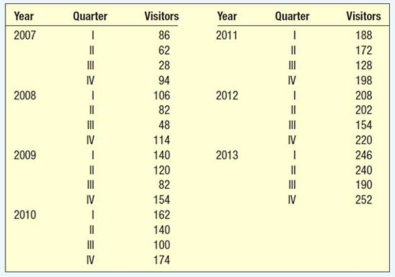
Ray Anderson, owner of Anderson Ski Lodge in upstate New York, is interested in forecasting the number of visitors for the upcoming year. The following data are available, by quarter, from the first quarter of 2007 to the fourth quarter of 2013. Develop a seasonal index for each quarter. How many visitors would you expect for each quarter of 2014, if Ray projects that there will be a 10% increase from the total number of visitors in 2013? Determine the trend equation, project the number of visitors for 2014, and seasonally adjust the forecast. Which forecast would you choose?
Obtain a seasonal index for each of the four quarters.
Find the number of visitors expected for each quarters of 2014 if there is 10% increase in the total number of visitors in 2013.
Obtain the trend equation.
Predict the number of visitors for 2014.
Find the seasonally adjusted forecasts.
Identify the best forecast.
Answer to Problem 33CE
The seasonal indexes for the four quarters are 1.2046, 1.0206, 0.6297, and 01.1451.
The number of visitors for each quarter of 2017 if there is 10% increase in the total number of visitors in 2013 is 255.25 visitors per quarter.
The trend equation is
The number of visitors for 2017 are 242.0171, 248.634, 255.2509, and 261.8678.
The seasonally adjusted forecasts are 291.5338, 253.7559, 160.7315, and 299.8648.
The best forecast is the fourth quarter of 2017.
Explanation of Solution
Four-year moving average:
Centered moving average:
Specific seasonal index:
| Year | Quarter | Visitors |
Four-quarter moving average |
Centered Moving average | Specific seasonal |
| 2007 | 1 | 86 | |||
| 2 | 62 | ||||
| 3 | 28 | 70 | 0.4 | ||
| 4 | 94 | 67.5 | 75 | 1.253333 | |
| 2008 | 1 | 106 | 72.5 | 80 | 1.325 |
| 2 | 82 | 77.5 | 85 | 0.964706 | |
| 3 | 48 | 82.5 | 91.75 | 0.523161 | |
| 4 | 114 | 87.5 | 100.75 | 1.131514 | |
| 2009 | 1 | 140 | 96 | 109.75 | 1.275626 |
| 2 | 120 | 105.5 | 119 | 1.008403 | |
| 3 | 82 | 114 | 126.75 | 0.646943 | |
| 4 | 154 | 124 | 132 | 1.166667 | |
| 2010 | 1 | 162 | 129.5 | 136.75 | 1.184644 |
| 2 | 140 | 134.5 | 141.5 | 0.989399 | |
| 3 | 100 | 139 | 147.25 | 0.679117 | |
| 4 | 174 | 144 | 154.5 | 1.126214 | |
| 2011 | 1 | 188 | 150.5 | 162 | 1.160494 |
| 2 | 172 | 158.5 | 168.5 | 1.020772 | |
| 3 | 128 | 165.5 | 174 | 0.735632 | |
| 4 | 198 | 171.5 | 180.25 | 1.098474 | |
| 2012 | 1 | 208 | 176.5 | 187.25 | 1.110814 |
| 2 | 202 | 184 | 193.25 | 1.045278 | |
| 3 | 154 | 190.5 | 200.75 | 0.767123 | |
| 4 | 220 | 196 | 210.25 | 1.046373 | |
| 2013 | 1 | 246 | 205.5 | 219.5 | 1.120729 |
| 2 | 240 | 215 | 228 | 1.052632 | |
| 3 | 190 | 224 | |||
| 4 | 252 | 232 |
The quarterly indexes are as follows:
| I | II | III | IV | |
| 2007 | 0.4 | 1.253333 | ||
| 2008 | 1.325 | 0.964706 | 0.523161 | 1.131514 |
| 2009 | 1.275626 | 1.008403 | 0.646943 | 1.166667 |
| 2010 | 1.184644 | 0.989399 | 0.679117 | 1.126214 |
| 2011 | 1.160494 | 1.020772 | 0.735632 | 1.098474 |
| 2012 | 1.110814 | 1.045278 | 0.767123 | 1.046373 |
| 2013 | 1.120729 | 1.052632 | ||
| Mean | 1.1962 | 1.0135 | 0.6253 | 1.1371 |
Seasonal index:
Here,
Therefore, the following is obtained:
The seasonal indexes are as follows:
| I | II | III | IV | |
| 2007 | 0.4 | 1.253333 | ||
| 2008 | 1.325 | 0.964706 | 0.523161 | 1.131514 |
| 2009 | 1.275626 | 1.008403 | 0.646943 | 1.166667 |
| 2010 | 1.184644 | 0.989399 | 0.679117 | 1.126214 |
| 2011 | 1.160494 | 1.020772 | 0.735632 | 1.098474 |
| 2012 | 1.110814 | 1.045278 | 0.767123 | 1.046373 |
| 2013 | 1.120729 | 1.052632 | ||
| Mean | 1.1962 | 1.0135 | 0.6253 | 1.1371 |
| Seasonal Index |
The total number of visitors in the year 2013 is
The 10% of 928 visitors is
The number of visitors in the year 2017 is
Therefore, the number of visitors in each quarter of 2017 is
Trend equation:
Step-by-step procedure to obtain the regression using the Excel:
- Enter the data for Year, Visitors and t in Excel sheet.
- Go to Data Menu.
- Click on Data Analysis.
- Select Regression and click on OK.
- Select the column of Visitors under Input Y Range.
- Select the column of t under Input X Range.
- Click on OK.
Output for the regression obtained using the Excel is as follows:
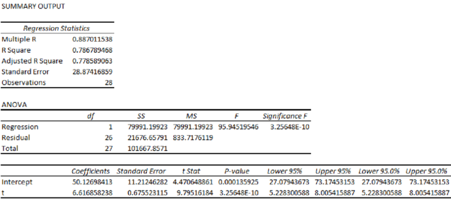
From the output, the regression equation is
Projection of the number of visitors for 2017:
The t value for the first quarter of 2014 is 29.
The t value for the second quarter of 2014 is 30.
The t value for the third quarter of 2014 is 31.
The t value for the fourth quarter of 2014 is 32.
Seasonally adjusted forecast:
| Estimated Visitors | Seasonal Index | |
| 242.0171 | 1.2046 | 291.5338 |
| 248.634 | 1.0206 | 253.7559 |
| 255.2509 | 0.6297 | 160.7315 |
| 261.8678 | 1.1451 | 299.8648 |
The seasonal index for the fourth quarter is high when compared to the remaining three quarters. Hence, the forecast for the fourth quarter is the best.
Want to see more full solutions like this?
Chapter 18 Solutions
Statistical Techniques in Business and Economics, 16th Edition


- C4 Q6 V1: Randomly collected student data in the dataset STATISTICSSTUDENTSSURVEYFORR contains the columns FEDBEST (preferred Federal party (Conservative, Green, Liberals, or NDP) ) , UNDERGORGRAD (degree being sought (GraduateProfessional, Undergraduate) ) and GENDERIDENTITY (Female or Male or Other). Make a crosstab (contingency) table of the counts for each of the (UNDERGORGRAD, FEDBEST) pairs for ONLY the females. If we randomly select a female student who is pursuing a graduateprofessional degree, what is the probability that she prefers the Federal Liberals. Choose the most correct (closest) answer below. Question 6 Answer a. 0.128 b. 0.263 c. 0.744 d. 0.333arrow_forwardInstall RStudio: Begin by installing RStudio on your computer. If you haven't done so, please refer to the official RStudio website for download and installation instructions. Watch the Tutorial Video: Watch the provided video tutorial that explains how to run RStudio. Pay close attention to the steps for opening and managing data files. https://www.youtube.com/watch?v=RhJp6vSZ7z0 Open RStudio: Once RStudio is installed, open the application. Load the Dataset: In RStudio, open a data file named "mtcars". To do this, type the command mtcars in the script editor and run the command. Attach the Data: Next, attach the dataset using the command attach(mtcars). Examine the Variables: Carefully review and note the names of all variables in the dataset. Examples of these variables include: Mileage (mpg) Number of Cylinders (cyl) Displacement (disp) Horsepower (hp) Research: Google to understand these variables. Statistical Analysis: Select mpg variable, and perform the following…arrow_forwardA marketing professor has surveyed the students at her university to better understand attitudes towards PPT usage for higher education. To be able to make inferences to the entire student body, the sample drawn needs to represent the university’s student population on all key characteristics. The table below shows the five key student demographic variables. The professor found the breakdown of the overall student body in the university’s fact book posted online. A non-parametric chi-square test was used to test the sample demographics against the population percentages shown in the table above. Review the output for the five chi-square tests on the following pages and answer the five questions: Based on the chi-square test, which sample variables adequately represent the university’s student population and which ones do not? Support your answer by providing the p-value of the chi-square test and explaining what it means. Using the results from Question 1, make recommendation for…arrow_forward
- A marketing professor has surveyed the students at her university to better understand attitudes towards PPT usage for higher education. To be able to make inferences to the entire student body, the sample drawn needs to represent the university’s student population on all key characteristics. The table below shows the five key student demographic variables. The professor found the breakdown of the overall student body in the university’s fact book posted online. A non-parametric chi-square test was used to test the sample demographics against the population percentages shown in the table above. Review the output for the five chi-square tests on the following pages and answer the five questions: Based on the chi-square test, which sample variables adequately represent the university’s student population and which ones do not? Support your answer by providing the p-value of the chi-square test and explaining what it means. Using the results from Question 1, make recommendation for…arrow_forwardA retail chain is interested in determining whether a digital video point-of-purchase (POP) display would stimulate higher sales for a brand advertised compared to the standard cardboard point-of-purchase display. To test this, a one-shot static group design experiment was conducted over a four-week period in 100 different stores. Fifty stores were randomly assigned to the control treatment (standard display) and the other 50 stores were randomly assigned to the experimental treatment (digital display). Compare the sales of the control group (standard POP) to the experimental group (digital POP). What were the average sales for the standard POP display (control group)? What were the sales for the digital display (experimental group)? What is the (mean) difference in sales between the experimental group and control group? List the null hypothesis being tested. Do you reject or retain the null hypothesis based on the results of the independent t-test? Was the difference between the…arrow_forwardWhat were the average sales for the four weeks prior to the experiment? What were the sales during the four weeks when the stores used the digital display? What is the mean difference in sales between the experimental and regular POP time periods? State the null hypothesis being tested by the paired sample t-test. Do you reject or retain the null hypothesis? At a 95% significance level, was the difference significant? Explain why or why not using the results from the paired sample t-test. Should the manager of the retail chain install new digital displays in each store? Justify your answer.arrow_forward
- A retail chain is interested in determining whether a digital video point-of-purchase (POP) display would stimulate higher sales for a brand advertised compared to the standard cardboard point-of-purchase display. To test this, a one-shot static group design experiment was conducted over a four-week period in 100 different stores. Fifty stores were randomly assigned to the control treatment (standard display) and the other 50 stores were randomly assigned to the experimental treatment (digital display). Compare the sales of the control group (standard POP) to the experimental group (digital POP). What were the average sales for the standard POP display (control group)? What were the sales for the digital display (experimental group)? What is the (mean) difference in sales between the experimental group and control group? List the null hypothesis being tested. Do you reject or retain the null hypothesis based on the results of the independent t-test? Was the difference between the…arrow_forwardQuestion 4 An article in Quality Progress (May 2011, pp. 42-48) describes the use of factorial experiments to improve a silver powder production process. This product is used in conductive pastes to manufacture a wide variety of products ranging from silicon wafers to elastic membrane switches. Powder density (g/cm²) and surface area (cm/g) are the two critical characteristics of this product. The experiments involved three factors: reaction temperature, ammonium percentage, stirring rate. Each of these factors had two levels, and the design was replicated twice. The design is shown in Table 3. A222222222222233 Stir Rate (RPM) Ammonium (%) Table 3: Silver Powder Experiment from Exercise 13.23 Temperature (°C) Density Surface Area 100 8 14.68 0.40 100 8 15.18 0.43 30 100 8 15.12 0.42 30 100 17.48 0.41 150 7.54 0.69 150 8 6.66 0.67 30 150 8 12.46 0.52 30 150 8 12.62 0.36 100 40 10.95 0.58 100 40 17.68 0.43 30 100 40 12.65 0.57 30 100 40 15.96 0.54 150 40 8.03 0.68 150 40 8.84 0.75 30 150…arrow_forward- + ++ Table 2: Crack Experiment for Exercise 2 A B C D Treatment Combination (1) Replicate I II 7.037 6.376 14.707 15.219 |++++ 1 བྱ॰༤༠སྦྱོ སྦྱོཋཏྟཱུ a b ab 11.635 12.089 17.273 17.815 с ас 10.403 10.151 4.368 4.098 bc abc 9.360 9.253 13.440 12.923 d 8.561 8.951 ad 16.867 17.052 bd 13.876 13.658 abd 19.824 19.639 cd 11.846 12.337 acd 6.125 5.904 bcd 11.190 10.935 abcd 15.653 15.053 Question 3 Continuation of Exercise 2. One of the variables in the experiment described in Exercise 2, heat treatment method (C), is a categorical variable. Assume that the remaining factors are continuous. (a) Write two regression models for predicting crack length, one for each level of the heat treatment method variable. What differences, if any, do you notice in these two equations? (b) Generate appropriate response surface contour plots for the two regression models in part (a). (c) What set of conditions would you recommend for the factors A, B, and D if you use heat treatment method C = +? (d) Repeat…arrow_forward
- Question 2 A nickel-titanium alloy is used to make components for jet turbine aircraft engines. Cracking is a potentially serious problem in the final part because it can lead to nonrecoverable failure. A test is run at the parts producer to determine the effect of four factors on cracks. The four factors are: pouring temperature (A), titanium content (B), heat treatment method (C), amount of grain refiner used (D). Two replicates of a 24 design are run, and the length of crack (in mm x10-2) induced in a sample coupon subjected to a standard test is measured. The data are shown in Table 2. 1 (a) Estimate the factor effects. Which factor effects appear to be large? (b) Conduct an analysis of variance. Do any of the factors affect cracking? Use a = 0.05. (c) Write down a regression model that can be used to predict crack length as a function of the significant main effects and interactions you have identified in part (b). (d) Analyze the residuals from this experiment. (e) Is there an…arrow_forwardA 24-1 design has been used to investigate the effect of four factors on the resistivity of a silicon wafer. The data from this experiment are shown in Table 4. Table 4: Resistivity Experiment for Exercise 5 Run A B с D Resistivity 1 23 2 3 4 5 6 7 8 9 10 11 12 I+I+I+I+Oooo 0 0 ||++TI++o000 33.2 4.6 31.2 9.6 40.6 162.4 39.4 158.6 63.4 62.6 58.7 0 0 60.9 3 (a) Estimate the factor effects. Plot the effect estimates on a normal probability scale. (b) Identify a tentative model for this process. Fit the model and test for curvature. (c) Plot the residuals from the model in part (b) versus the predicted resistivity. Is there any indication on this plot of model inadequacy? (d) Construct a normal probability plot of the residuals. Is there any reason to doubt the validity of the normality assumption?arrow_forwardStem1: 1,4 Stem 2: 2,4,8 Stem3: 2,4 Stem4: 0,1,6,8 Stem5: 0,1,2,3,9 Stem 6: 2,2 What’s the Min,Q1, Med,Q3,Max?arrow_forward
 Glencoe Algebra 1, Student Edition, 9780079039897...AlgebraISBN:9780079039897Author:CarterPublisher:McGraw Hill
 Trigonometry (MindTap Course List)TrigonometryISBN:9781305652224Author:Charles P. McKeague, Mark D. TurnerPublisher:Cengage Learning
 Holt Mcdougal Larson Pre-algebra: Student Edition...AlgebraISBN:9780547587776Author:HOLT MCDOUGALPublisher:HOLT MCDOUGAL
 College Algebra (MindTap Course List)AlgebraISBN:9781305652231Author:R. David Gustafson, Jeff HughesPublisher:Cengage Learning
 Big Ideas Math A Bridge To Success Algebra 1: Stu...AlgebraISBN:9781680331141Author:HOUGHTON MIFFLIN HARCOURTPublisher:Houghton Mifflin Harcourt