Chapter 18, Problem 31CE

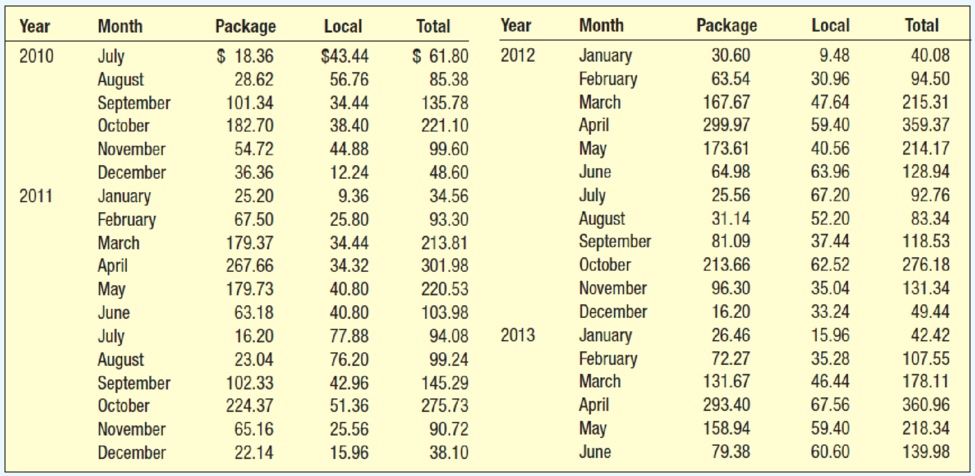
Blueberry Farms Golf and Fish Club of Hilton Head, South Carolina, wants to find monthly seasonal indexes for package play, nonpackage play, and total play. The package play refers to golfers who visit the area as part of a golf package. Typically, the greens fees, cart fees, lodging, maid service, and meals are included as part of a golfing package. The course earns a certain percentage of this total. The nonpackage play includes play by local residents and visitors to the area who wish to play golf. The following data, beginning with July 2010 and ending with June 2013, report the package and nonpackage play by month, as well as the total amount, in thousands of dollars.

Using statistical software:

1. a. Develop a seasonal index for each month for the package sales. What do you note about the various months?
2. b. Develop a seasonal index for each month for the nonpackage sales. What do you note about the various months?
3. c. Develop a seasonal index for each month for the total sales. What do you note about the various months?
4. d. Compare the indexes for package sales, nonpackage sales, and total sales. Are the busiest months the same?

To determine

Provide a seasonal index for each month for the package sales.

Write a note about the seasonal index for package sales of various months.

Answer to Problem 31CE

The seasonal indexes for each month for the package sales are given below:

Period	Month	Seasonal Index
1	July	0.19792
2	August	0.25663
3	September	0.8784
4	October	2.10481
5	November	0.77747
6	December	0.18388
7	January	0.26874
8	February	0.63189
9	March	1.67943
10	April	2.73547
11	May	1.67903
12	June	0.60633

The two months, October and April signify more than twice the average.

Explanation of Solution

Twelve months moving average:

$\text{Twelve-year moving average}=\frac{\text{sum of the twelve concequent packages}}{12}$.

Centered moving average:

$\text{Centered moving average}=\frac{\text{sum of the two concequent moving averages}}{2}$.

Specific seasonal index:

$\text{Specific seasonal index}=\frac{\text{packages}}{\text{Centered moving average}}$

Some preliminary calculations are given below:

Year	Quarter	Package	Four-quarter moving average	Centered Moving average	Specific seasonal
2010	July	18.36
	August	28.62
	September	101.34
	October	182.7
	November	54.72
	December	36.36
2011	January	25.2		100.305	0.25123
	February	67.5	100.395	99.9825	0.67512
	March	179.37	100.215	99.79125	1.79745
	April	267.66	99.75	101.5688	2.63526
	May	179.73	99.8325	103.74	1.73250
	June	63.18	103.305	103.5825	0.60995
	July	16.2	104.175	103.215	0.15695
	August	23.04	102.99	103.275	0.22309
	September	102.33	103.44	102.6225	0.99715
	October	224.37	103.11	103.4813	2.16822
	November	65.16	102.135	104.5725	0.62311
	December	22.14	104.8275	104.3925	0.21209
2012	January	30.6	104.3175	104.8575	0.29183
	February	63.54	104.4675	105.585	0.60179
	March	167.67	105.2475	105.0375	1.59629
	April	299.97	105.9225	103.7063	2.89249
	May	173.61	104.1525	104.5575	1.66042
	June	64.98	103.26	105.6075	0.61529
	July	25.56	105.855	105.1875	0.24299
	August	31.14	105.36	105.3788	0.29551
	September	81.09	105.015	104.2425	0.77789
	October	213.66	105.7425	102.4688	2.08512
	November	96.3	102.7425	101.5838	0.94799
	December	16.2	102.195	101.5725	0.15949
2013	January	26.46	100.9725
	February	72.27	102.1725
	March	131.67	109.1373
	April	293.4	116.937
	May	158.94	120.92
	June	79.38	109.3275

The monthly indexes are as follows:

	2010	2011	2012	2013	Means
Jan	-	0.25123	0.29183	-	0.27153
Feb	-	0.67512	0.60179	-	0.63845
Mar	-	1.79745	1.59629	-	1.69687
April	-	2.63526	2.89249	-	2.76388
May	-	1.7325	1.66042	-	1.69647
June	-	0.60995	0.61529	-	0.61262
July	-	0.15695	0.24299	-	0.19997
August	-	0.22309	0.29551	-	0.25929
Sep	-	0.99715	0.7778	-	0.88752
Oct	-	2.16822	2.0851	-	2.12667
Nov	-	0.6231	0.9479	-	0.78555
Dec	-	0.21208	0.1594	-	0.18579
Total					12.1246233

Seasonal index:

$\text{Seasonal Index}=\text{Mean of the Month}\times \text{Correction Factor}$

Here, $\text{Correction Factor}=\frac{12}{\text{Sum of the means of the months}}$.

Therefore, the following is obtained:

$\begin{array}{c}\text{Correction Factor}=\frac{12}{12.1246233}\\ =0.98972147\end{array}$

The seasonal indexes are as follows:

	2010	2011	2012	2013	Means	Seasonal Index
Jan	-	0.25123	0.29183	-	0.27153	0.268738257
Feb	-	0.67512	0.60179	-	0.63845	0.631891717
Mar	-	1.79745	1.59629	-	1.69687	1.679428286
April	-	2.63526	2.89249	-	2.76388	2.735469498
May	-	1.7325	1.66042	-	1.69647	1.679028041
June	-	0.60995	0.61529	-	0.61262	0.606326037
July	-	0.15695	0.24299	-	0.19997	0.19791885
August	-	0.22309	0.29551	-	0.25929	0.256634371
Sep	-	0.99715	0.7778	-	0.88752	0.87840128
Oct	-	2.16822	2.0851	-	2.12667	2.104812143
Nov	-	0.6231	0.9479	-	0.78555	0.777473047
Dec	-	0.21208	0.1594	-	0.18579	0.183878466

The seasonal index for October is 2.10481 and the seasonal index for April is 2.73547. That is, the months October and April represent more than twice the average when compared to other months.

To determine

Create a seasonal index for each month for the non-package sales.

Write a note on seasonal index for the non-package sales for various months.

Answer to Problem 31CE

The seasonal index for each month for the non-package sales are as follows:

Period	Month	Seasonal Index
1	July	1.73270
2	August	1.53389
3	September	0.94145
4	October	1.29183
5	November	0.66928
6	December	0.52991
7	January	0.23673
8	February	0.69732
9	March	1.00695
10	April	1.13226
11	May	0.98282
12	June	1.24486

The two months, December and January have the low index values.

Explanation of Solution

The specific seasonal indices are as follows:

Year	Quarter	Local ($)	Four-quarter moving average	Centered Moving average	Specific seasonal
2010	July	43.44
	August	56.76
	September	34.44
	October	38.4
	November	44.88
	December	12.24
2011	January	9.36		36.075	0.259459
	February	25.8	34.64	38.32	0.673278
	March	34.44	37.51	39.485	0.87223
	April	34.32	39.13	40.38	0.849926
	May	40.8	39.84	40.115	1.017076
	June	40.8	40.92	39.465	1.033827
	July	77.88	39.31	39.625	1.965426
	August	76.2	39.62	39.845	1.912411
	September	42.96	39.63	40.61	1.057868
	October	51.36	40.06	42.205	1.216917
	November	25.56	41.16	43.24	0.591119
	December	15.96	43.25	44.195	0.361127
2012	January	9.48	43.23	44.715	0.212009
	February	30.96	45.16	43.27	0.715507
	March	47.64	44.27	42.04	1.133206
	April	59.4	42.27	42.275	1.405086
	May	40.56	41.81	43.135	0.940304
	June	63.96	42.74	44.25	1.445424
	July	67.2	43.53	45.24	1.485411
	August	52.2	44.97	45.69	1.142482
	September	37.44	45.51	45.82	0.81711
	October	62.52	45.87	46.11	1.355888
	November	35.04	45.77	47.235	0.741823
	December	33.24	46.45	47.88	0.694236
2013	January	15.96	48.02
	February	35.28	47.74
	March	46.44	45.97091
	April	67.56	45.348
	May	59.4	46.22667
	June	60.6	44.19

The monthly indexes are as follows:

	2010	2011	2012	2013	Means
Jan	-	0.25123	0.29183	-	0.235734
Feb	-	0.67512	0.60179	-	0.694392
Mar	-	1.79745	1.59629	-	1.002718
April	-	2.63526	2.89249	-	1.127506
May	-	1.7325	1.66042	-	0.97869
June	-	0.60995	0.61529	-	1.239626
July	-	0.15695	0.24299	-	1.725419
August	-	0.22309	0.29551	-	1.527446
Sep	-	0.99715	0.7778	-	0.937489
Oct	-	2.16822	2.0851	-	1.286403
Nov	-	0.6231	0.9479	-	0.666471
Dec	-	0.21208	0.1594	-	0.527681
Total					11.94958

The $\text{Correction Factor}=\frac{12}{\text{Sum of the means of the months}}$.

Therefore, the following is obtained:

$\begin{array}{c}\text{Correction Factor}=\frac{12}{11.94958}\\ =1.00422\end{array}$

The seasonal indexes are as follows:

	2010	2011	2012	2013	Means	Seasonal Index
Jan	-	0.25123	0.29183	-	0.235734	0.23673
Feb	-	0.67512	0.60179	-	0.694392	0.69732
Mar	-	1.79745	1.59629	-	1.002718	1.00695
April	-	2.63526	2.89249	-	1.127506	1.13226
May	-	1.7325	1.66042	-	0.97869	0.98282
June	-	0.60995	0.61529	-	1.239626	1.24486
July	-	0.15695	0.24299	-	1.725419	1.73270
August	-	0.22309	0.29551	-	1.527446	1.53389
Sep	-	0.99715	0.7778	-	0.937489	0.94145
Oct	-	2.16822	2.0851	-	1.286403	1.29183
Nov	-	0.6231	0.9479	-	0.666471	0.66928
Dec	-	0.21208	0.1594	-	0.527681	0.52991

The seasonal index for December is 0.52991 and the seasonal index for January is 0.23673. That is, the months December and January represent the less index values when compared to other months.

To determine

Create a seasonal index for each month for the total sales.

Write a note on various months.

Answer to Problem 31CE

The seasonal indexes for each month for the total sales are as follows:

Period	Month	Seasonal Index
1	July	0.63371
2	August	0.61870
3	September	0.89655
4	October	1.86415
5	November	0.74353
6	December	0.29180
7	January	0.25908
8	February	0.65069
9	March	1.49028
10	April	2.28041
11	May	1.48235
12	June	0.78876

The two months December and January have the low index values.

The two months April and October have the high index values.

Explanation of Solution

The specific seasonal indices are as follows:

Year	Quarter	Local ($)	Four-quarter moving average	Centered Moving average	Specific seasonal
2010	July	61.8
	August	85.38
	September	135.78
	October	221.1
	November	99.6
	December	48.6
2011	January	34.56		136.38	0.270833
	February	93.3	135.035	138.3025	0.276527
	March	213.81	137.725	139.2763	0.161078
	April	301.98	138.88	141.9488	0.11365
	May	220.53	139.6725	143.855	0.185009
	June	103.98	144.225	143.0475	0.392383
	July	94.08	143.485	142.84	0.827806
	August	99.24	142.61	143.12	0.767836
	September	145.29	143.07	143.2325	0.295684
	October	275.73	143.17	145.6863	0.186269
	November	90.72	143.295	147.8125	0.281746
	December	38.1	148.0775	148.5875	0.418898
2012	January	40.08	147.5475	149.5725	0.236527
	February	94.5	149.6275	148.855	0.327619
	March	215.31	149.5175	147.0775	0.221262
	April	359.37	148.1925	145.9813	0.165289
	May	214.17	145.9625	147.6925	0.189382
	June	128.94	146	149.8575	0.496045
	July	92.76	149.385	150.4275	0.72445
	August	83.34	150.33	151.0688	0.62635
	September	118.53	150.525	150.0625	0.315869
	October	276.18	151.6125	148.5788	0.226374
	November	131.34	148.5125	148.8188	0.266788
	December	49.44	148.645	149.4525	0.67233
2013	January	42.42	148.9925
	February	107.55	149.9125
	March	178.11	155.1082
	April	360.96	162.285
	May	218.34	167.1467
	June	139.98	153.5175

The monthly indexes are given below:

	2010	2011	2012	2013	Means
Jan	-	0.25341	0.267964	-	0.260687
Feb	-	0.674608	0.634846	-	0.654727
Mar	-	1.53515	1.463922	-	1.499536
April	-	2.127388	2.461755	-	2.294571
May	-	1.533002	1.450107	-	1.491555
June	-	0.726891	0.860417	-	0.793654
July	-	0.658639	0.616643	-	0.637641
August	-	0.693404	0.551669	-	0.622537
Sep	-	1.014365	0.789871	-	0.902118
Oct	-	1.892629	1.858812	-	1.875721
Nov	-	0.613751	0.88255	-	0.74815
Dec	-	0.256415	0.330807	-	0.293611
Total					0.993829

The $\text{Correction Factor}=\frac{12}{\text{Sum of the means of the months}}$

Therefore, the following is obtained:

$\begin{array}{c}\text{Correction Factor}=\frac{12}{12.07451}\\ =0.993829\end{array}$

The seasonal indexes are given below:

	2010	2011	2012	2013	Means	Seasonal Index
Jan	-	0.25341	0.267964		0.260687	0.25908
Feb	-	0.674608	0.634846		0.654727	0.65069
Mar	-	1.53515	1.463922		1.499536	1.49028
April	-	2.127388	2.461755		2.294571	2.28041
May	-	1.533002	1.450107		1.491555	1.48235
June	-	0.726891	0.860417		0.793654	0.78876
July	-	0.658639	0.616643		0.637641	0.63371
August	-	0.693404	0.551669		0.622537	0.61870
Sep	-	1.014365	0.789871		0.902118	0.89655
Oct	-	1.892629	1.858812		1.875721	1.86415
Nov	-	0.613751	0.88255		0.74815	0.74353
Dec	-	0.256415	0.330807		0.293611	0.29180

The seasonal index for January is 0.25908 and the seasonal index for December is 0.29180. That is, the months December and January represent the less index values when compared to other months. The seasonal index for April is 2.28041 and the seasonal index for October is 1.86415. That is, the months April and October represent the more index values when compared to other months.

To determine

Compare the indexes for package sales, non-package sales, and total sales.

Explain whether the busiest months are all the same.

Explanation of Solution

The seasonal index for April in package play is large when compared to remaining months. Hence, the package play is the highest in April.

The seasonal index for July in non-package is large when compared to the remaining months. Hence, the non-package play is the highest play in July. From the given information, 70% of the total sales come from package play. Hence, the total play is very similar to package play.