Videos
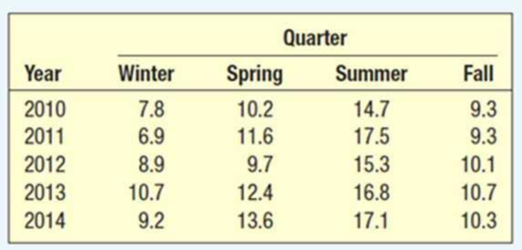
The quarterly production of pine lumber, in millions of board feet, by Northwest Lumber for 2010 through 2014 is:
- a. Determine the typical seasonal pattern for the production data using the ratio-to-moving-average method.
- b. Interpret the pattern.
- c. Deseasonalize the data and determine the linear trend equation.
- d. Project the seasonally adjusted production for the four quarters of 2015.
a.
Obtain the typical seasonal patterns for the production data using the ratio-to-moving-average method.
Answer to Problem 28CE
The typical seasonal patterns for sales are 0.7549, 0.9913, 1.4043, and 0.8495.
Explanation of Solution
Four-year moving average:
Centered moving average:
Specific seasonal index:
| Year | Quarter | Board ft Millions |
Four-quarter moving average |
Centered Moving average | Specific seasonal |
| 2010 | Winter | 7.8 | |||
| Spring | 10.2 | ||||
| Summer | 14.7 | 10.3875 | 1.41516 | ||
| Fall | 9.3 | 10.5 | 10.45 | 0.88995 | |
| 2011 | Winter | 6.9 | 10.275 | 10.975 | 0.6287 |
| Spring | 11.6 | 10.625 | 11.325 | 1.02428 | |
| Summer | 17.5 | 11.325 | 11.575 | 1.51188 | |
| Fall | 9.3 | 11.325 | 11.5875 | 0.80259 | |
| 2012 | Winter | 8.9 | 11.825 | 11.075 | 0.80361 |
| Spring | 9.7 | 11.35 | 10.9 | 0.88991 | |
| Summer | 15.3 | 10.8 | 11.225 | 1.36303 | |
| Fall | 10.1 | 11 | 11.7875 | 0.85684 | |
| 2013 | Winter | 10.7 | 11.45 | 12.3125 | 0.86904 |
| Spring | 12.4 | 12.125 | 12.575 | 0.98608 | |
| Summer | 16.8 | 12.5 | 12.4625 | 1.34804 | |
| Fall | 10.7 | 12.65 | 12.425 | 0.86117 | |
| 2014 | Winter | 9.2 | 12.275 | 12.6125 | 0.72944 |
| Spring | 13.6 | 12.575 | 12.6 | 1.07937 | |
| Summer | 17.1 | 12.65 | |||
| Fall | 10.3 | 12.55 |
The quarterly indexes are as follows:
| Winter | Spring | Summer | Fall | |
| 2010 | 1.415162 | 0.889952 | ||
| 2011 | 0.628702 | 1.024283 | 1.511879 | 0.802589 |
| 2012 | 0.803612 | 0.889908 | 1.363029 | 0.85684 |
| 2013 | 0.869036 | 0.986083 | 1.348044 | 0.861167 |
| 2014 | 0.729435 | 1.079365 | ||
| Mean | 0.757696 | 0.99491 | 1.409529 | 0.852637 |
Typical seasonal index:
Here,
Therefore, the following is obtained:
The typical seasonal indexes are as follows:
| Winter | Spring | Summer | Fall | |
| 2010 | 1.415162 | 0.889952 | ||
| 2011 | 0.628702 | 1.024283 | 1.511879 | 0.802589 |
| 2012 | 0.803612 | 0.889908 | 1.363029 | 0.85684 |
| 2013 | 0.869036 | 0.986083 | 1.348044 | 0.861167 |
| 2014 | 0.729435 | 1.079365 | ||
| Mean | 0.757696 | 0.99491 | 1.409529 | 0.852637 |
| Typical Index | 0.7549 | 0.9913 | 1.4043 | 0.8495 |
b.
Interpret the typical seasonal pattern.
Explanation of Solution
The typical seasonal index for the summer quarter is 1.4043, which is the largest compared to the other three quarters. That is, the production is the largest in the third quarter and moreover, it represents above the average quarters because the corresponding seasonal index is greater than 1. The winter, spring, and fall quarters represent below the average quarters because seasonal indexes for the three quarters are less than 1.
c.
Determine the trend equation.
Answer to Problem 28CE
The trend equation is
Explanation of Solution
Calculation:
Deseasonalization:
| Board ft Millions | Typical Seasonal Index | Deseasonalized production |
| 7.8 | 0.7549 | 10.33249437 |
| 10.2 | 0.9913 | 10.28951881 |
| 14.7 | 1.4043 | 10.46784875 |
| 9.3 | 0.8495 | 10.94761624 |
| 6.9 | 0.7549 | 9.140283481 |
| 11.6 | 0.9913 | 11.70180571 |
| 17.5 | 1.4043 | 12.4617247 |
| 9.3 | 0.8495 | 10.94761624 |
| 8.9 | 0.7549 | 11.78964101 |
| 9.7 | 0.9913 | 9.785130637 |
| 15.3 | 1.4043 | 10.89510788 |
| 10.1 | 0.8495 | 11.88934667 |
| 10.7 | 0.7549 | 14.17406279 |
| 12.4 | 0.9913 | 12.50882679 |
| 16.8 | 1.4043 | 11.96325571 |
| 10.7 | 0.8495 | 12.5956445 |
| 9.2 | 0.7549 | 12.18704464 |
| 13.6 | 0.9913 | 13.71935842 |
| 17.1 | 1.4043 | 12.17688528 |
| 10.3 | 0.8495 | 12.12477928 |
Assign t value as 1 for the first quarter of 2010, 2 for the second quarter of 2010, and so on.
Step-by-step procedure to obtain the regression using the Excel:
- Enter the data for Deseasonalized production and t in Excel sheet.
- Go to Data Menu.
- Click on Data Analysis.
- Select Regression and click on OK.
- Select the column of Deseasonalized production under Input Y Range.
- Select the column of t under Input X Range.
- Click on OK.
Output for the regression obtained using the Excel is as follows:
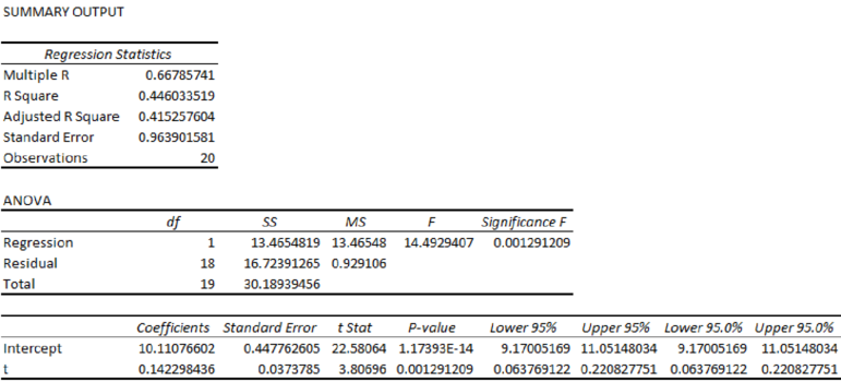
From the Excel output, the regression equation is
d.
Find the seasonally adjusted production for the four quarters of 2017.
Answer to Problem 28CE
The seasonally adjusted production for the four quarters of 2017 are 9.8884, 13.1261, 18.7946, and 11.4903.
Explanation of Solution
From the output, the regression equation is
The t value for the first quarter of 2017 is 21.
The t value for the second quarter of 2017 is 22.
The t value for the third quarter of 2017 is 23.
The t value for the fourth quarter of 2017 is 24.
Seasonally adjusted forecast:
| Estimated Visitors | Seasonal Index | |
| 13.0990 | 0.7549 | 9.8884 |
| 13.2413 | 0.9913 | 13.1261 |
| 13.3836 | 1.4043 | 18.7946 |
| 13.5259 | 0.8495 | 11.4903 |
Want to see more full solutions like this?
Chapter 18 Solutions
Statistical Techniques in Business and Economics


- Examine the Variables: Carefully review and note the names of all variables in the dataset. Examples of these variables include: Mileage (mpg) Number of Cylinders (cyl) Displacement (disp) Horsepower (hp) Research: Google to understand these variables. Statistical Analysis: Select mpg variable, and perform the following statistical tests. Once you are done with these tests using mpg variable, repeat the same with hp Mean Median First Quartile (Q1) Second Quartile (Q2) Third Quartile (Q3) Fourth Quartile (Q4) 10th Percentile 70th Percentile Skewness Kurtosis Document Your Results: In RStudio: Before running each statistical test, provide a heading in the format shown at the bottom. “# Mean of mileage – Your name’s command” In Microsoft Word: Once you've completed all tests, take a screenshot of your results in RStudio and paste it into a Microsoft Word document. Make sure that snapshots are very clear. You will need multiple snapshots. Also transfer these results to the…arrow_forward2 (VaR and ES) Suppose X1 are independent. Prove that ~ Unif[-0.5, 0.5] and X2 VaRa (X1X2) < VaRa(X1) + VaRa (X2). ~ Unif[-0.5, 0.5]arrow_forward8 (Correlation and Diversification) Assume we have two stocks, A and B, show that a particular combination of the two stocks produce a risk-free portfolio when the correlation between the return of A and B is -1.arrow_forward
- 9 (Portfolio allocation) Suppose R₁ and R2 are returns of 2 assets and with expected return and variance respectively r₁ and 72 and variance-covariance σ2, 0%½ and σ12. Find −∞ ≤ w ≤ ∞ such that the portfolio wR₁ + (1 - w) R₂ has the smallest risk.arrow_forward7 (Multivariate random variable) Suppose X, €1, €2, €3 are IID N(0, 1) and Y2 Y₁ = 0.2 0.8X + €1, Y₂ = 0.3 +0.7X+ €2, Y3 = 0.2 + 0.9X + €3. = (In models like this, X is called the common factors of Y₁, Y₂, Y3.) Y = (Y1, Y2, Y3). (a) Find E(Y) and cov(Y). (b) What can you observe from cov(Y). Writearrow_forward1 (VaR and ES) Suppose X ~ f(x) with 1+x, if 0> x > −1 f(x) = 1−x if 1 x > 0 Find VaRo.05 (X) and ES0.05 (X).arrow_forward
- Joy is making Christmas gifts. She has 6 1/12 feet of yarn and will need 4 1/4 to complete our project. How much yarn will she have left over compute this solution in two different ways arrow_forwardSolve for X. Explain each step. 2^2x • 2^-4=8arrow_forwardOne hundred people were surveyed, and one question pertained to their educational background. The results of this question and their genders are given in the following table. Female (F) Male (F′) Total College degree (D) 30 20 50 No college degree (D′) 30 20 50 Total 60 40 100 If a person is selected at random from those surveyed, find the probability of each of the following events.1. The person is female or has a college degree. Answer: equation editor Equation Editor 2. The person is male or does not have a college degree. Answer: equation editor Equation Editor 3. The person is female or does not have a college degree.arrow_forward
 Glencoe Algebra 1, Student Edition, 9780079039897...AlgebraISBN:9780079039897Author:CarterPublisher:McGraw Hill
 Holt Mcdougal Larson Pre-algebra: Student Edition...AlgebraISBN:9780547587776Author:HOLT MCDOUGALPublisher:HOLT MCDOUGAL
 Trigonometry (MindTap Course List)TrigonometryISBN:9781305652224Author:Charles P. McKeague, Mark D. TurnerPublisher:Cengage Learning
 College Algebra (MindTap Course List)AlgebraISBN:9781305652231Author:R. David Gustafson, Jeff HughesPublisher:Cengage Learning
 Functions and Change: A Modeling Approach to Coll...AlgebraISBN:9781337111348Author:Bruce Crauder, Benny Evans, Alan NoellPublisher:Cengage Learning