
Concept explainers
Videos
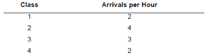
A priority waiting system assigns arriving customers to one of four classes. Arrival rates (Poisson) of the classes are shown in the following table. Five servers process the customers, and each can handle three customers per hour.
a. What is the system utilization?
b. What is the average wait for service by customers in the various classes? How many are waiting in each class, on average?
c. If the arrival rate of the second priority class could be reduced to three units per hour by shifting some arrivals into the third priority class, how would your answers to part b change?
d. What observations can you make based on your answers to part c?
a)
To determine: System utilization rate.
Introduction: Poisson distribution is utilized to ascertain the probability of an occasion happening over a specific time period or interval. The interval can be one of time, zone, volume or separation. The probability of an event happening is discovered utilizing the equation in the Poisson distribution.
Answer to Problem 16P
Explanation of Solution
Given Information:
It is given that the processing time is 3 customers per hour and there are 5 servers to process the customers.
| Class | Arrivals per Hour |
| 1 | 2 |
| 2 | 4 |
| 3 | 3 |
| 4 | 2 |
Calculate the system utilization:
It is calculated by adding all the total customer hours for each class and the result is divided with number of servers and customer process per hour.
ρ=[λ1+λ2+λ3+λ4Mμ]=[2+4+3+25×3]=[11 per hour15]=0.7333 per hour
Here,
ρ = system utilization rate
λ1 = total customer arrival rate for class 1
λ2 = total customer arrival rate for class 2
λ3 = total customer arrival rate for class 3
λ4 = total customer arrival rate for class 4
μ = customer service process rate per hour
M = number of servers
Hence the system utilization is 0.7333.
b)
To determine: The average customer waiting for service for each class and waiting in each class on average.
Answer to Problem 16P
Explanation of Solution
Given Information:
It is given that the processing time is 3 customers per hour and there are 5 servers to process the customers.
| Class | Arrivals per Hour |
| 1 | 2 |
| 2 | 4 |
| 3 | 3 |
| 4 | 2 |
Calculate the average number of customers:
It is calculated by dividing the total customers arrive per hour with customer process per hour.
r=[λμ]=[113]=3.6667
Here,
r = average number of customers
λ= total customer arrival rate
μ = customer service process rate per hour
Calculate average number of customers waiting for service (Lq) using infinite-source table values for μ= 3.6667 and M = 5
The Lq values for μ= 3.6667 and M = 5 is 1.1904
Calculate A using Formula 18-16 from book:
It is calculated by subtracting 1 minus system utilization rate and multiplying the result with Lq, the whole result is divided by total customer arrival rate.
A=[λ1+λ2+λ3+λ4(1−ρ)Lq]=[2+4+3+2(1−0.7333)×1.1904]=[110.2667×1.1904]=[110.31744]=34.6522
Here,
Lq = average number of customers waiting for service
λ1 = total customer arrival rate for class 1
λ2 = total customer arrival rate for class 2
λ3 = total customer arrival rate for class 3
λ4 = total customer arrival rate for class 4
ρ = system utilization rate
Calculate B using Formula 18-17 from book for each category
It is calculated by multiplying number of servers with customer service process rate per hour and the result is divided by total customer arrival rate for each category.
B0=1B1=[1−(λ1Mμ)]=[1−(25×3)]=[1−(215)]=[1−0.1333]=0.8667
B2=[1−(λ1+λ2Mμ)]=[1−(2+45×3)]=[1−(615)]=[1−0.4000]=0.6000
B3=[1−(λ1+λ2+λ3Mμ)]=[1−(2+4+35×3)]=[1−(915)]=[1−0.6000]=0.4000
B4=[1−(λ1+λ2+λ3+λ4Mμ)]=[1−(2+4+3+25×3)]=[1−(1115)]=[1−0.7333]=0.2667
Here,
λ1= total customer arrival rate for class 1
λ2= total customer arrival rate for class 2
λ3= total customer arrival rate for class 3
λ4= total customer arrival rate for class 4
μ = customer service process rate per hour
M = number of servers
B1= total customer arrival rate for class 1
B2= total customer arrival rate for class 2
B3= total customer arrival rate for class 1
B4= total customer arrival rate for class 2
Calculate the average waiting time for class 1 and class 2
It is calculated by multiplying A with B0 and B1, the result is divided by 1.
W1=[1A×B0×B1]=[134.6522×1×0.8667]=[130.0319]=0.033298 or 0.0333 hours
W2=[1A×B1×B2]=[134.6522×0.8667×0.6]=[118.0192]=0.055497 or 0.0555 hours
W3=[1A×B2×B3]=[134.6522×0.6×0.4]=[18.3165]=0.120242 or 0.1202 hours
W4=[1A×B3×B4]=[134.6522×0.4×0.2667]=[13.6962]=0.270545 or 0.2705 hours
Calculate the average number of customers that are waiting for service for class 1 and class 2:
It is calculated by multiplying total customer arrival rate with average waiting time for units in each category.
L1=[W1×λ1]=[0.033298×2]=0.066596 or 0.0666 customers
L2=[W2×λ2]=[0.055497×4]=0.221986 or 0.2220 customers
L3=[W3×λ3]=[0.120242×3]=0.360727 or 0.3607 customers
L4=[W4×λ4]=[0.270545×2]=0.541091 or 0.5411 customers
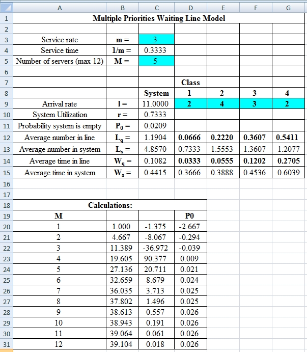
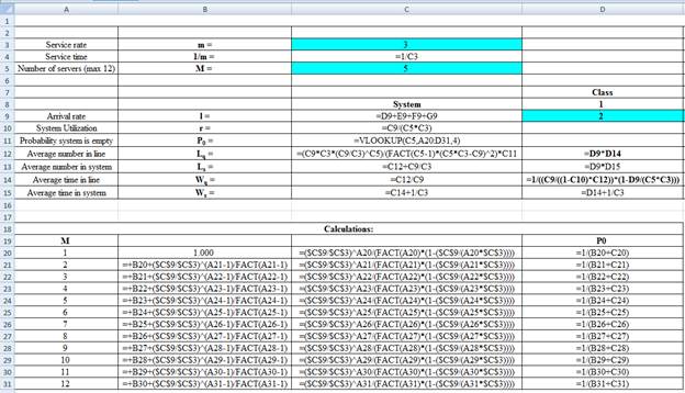
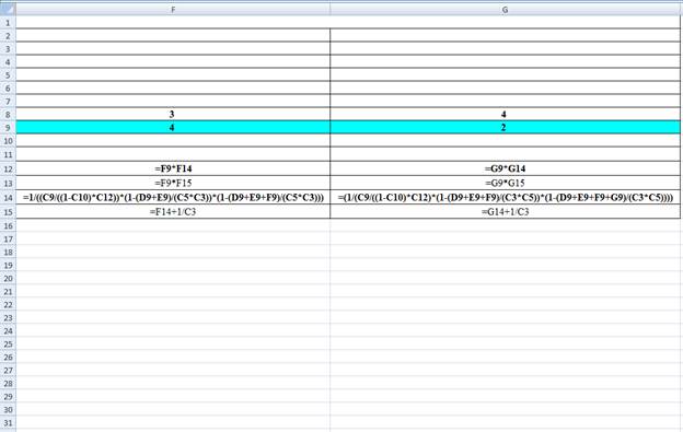
Excel Spreadsheet:
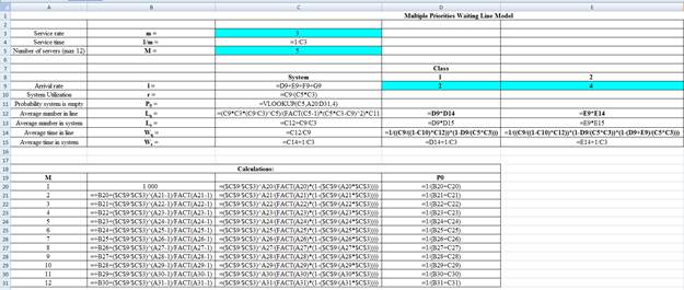
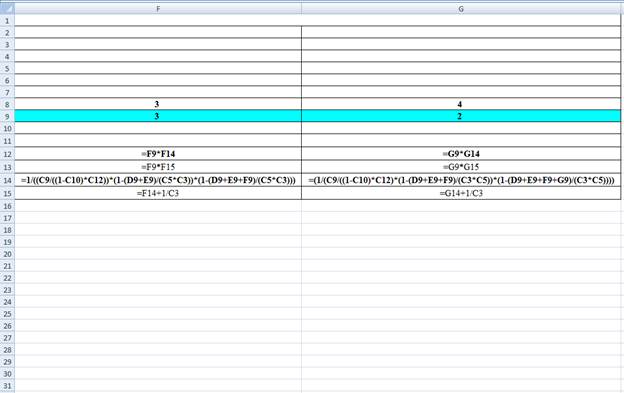
Excel Workings:
Hence the average wait time for service by customers for class 1 is 0.0333 hours, class 2 is 0.0555 hours, class 3 is 0.1202 hours and class 4 is 0.2705 hours. The waiting in each class on average for class 1 is 0.0666 customers, class 2 is 0.2220 customers, class 3 is 0.3607 customers and class 4 is 0.5411 customers.
c)
To determine: The average customer waiting for service for each class and waiting in each class on average.
Answer to Problem 16P
Explanation of Solution
Given Information:
It is given that the processing time is 3 customers per hour and there are 5 servers to process the customers. The second priority class is reduced to 3 units per hour by shifting some into the third party class. The arrival rate is as follows,
| Class | Arrivals per Hour |
| 1 | 2 |
| 2 | 3 |
| 3 | 4 |
| 4 | 2 |
Calculate the average number of customers
It is calculated by dividing the total customers arrive per hour with customer process per hour.
r=[λμ]=[113]=3.6667
Here,
r = average number of customers
λ= total customer arrival rate
μ = customer service process rate per hour
Calculate average number of customers waiting for service (Lq) using infinite-source table values for μ= 3.6667 and M = 5
The Lq values for μ= 3.6667 and M = 5 is 1.1904
Calculate A using Formula 18-16 from book:
It is calculated by subtracting 1 minus system utilization rate and multiplying the result with Lq, the whole result is divided by total customer arrival rate.
A=[λ1+λ2+λ3+λ4(1−ρ)Lq]=[2+3+4+2(1−0.7333)×1.1904]=[110.2667×1.1904]=[110.31744]=34.6522
Here,
Lq = average number of customers waiting for service
λ1 = total customer arrival rate for class 1
λ2 = total customer arrival rate for class 2
λ3 = total customer arrival rate for class 3
λ4 = total customer arrival rate for class 4
ρ = system utilization rate
Calculate B using Formula 18-17 from book for each category
It is calculated by multiplying number of servers with customer service process rate per hour and the result is divided by total customer arrival rate for each category.
B0=1B1=[1−(λ1Mμ)]=[1−(25×3)]=[1−(215)]=[1−0.1333]=0.8667
B2=[1−(λ1+λ2Mμ)]=[1−(2+35×3)]=[1−(515)]=[1−0.3333]=0.6667
B3=[1−(λ1+λ2+λ3Mμ)]=[1−(2+3+45×3)]=[1−(915)]=[1−0.6000]=0.4000
B4=[1−(λ1+λ2+λ3+λ4Mμ)]=[1−(2+3+4+25×3)]=[1−(1115)]=[1−0.7333]=0.2667
Here,
λ1= total customer arrival rate for class 1
λ2= total customer arrival rate for class 2
λ3= total customer arrival rate for class 3
λ4= total customer arrival rate for class 4
μ = customer service process rate per hour
M = number of servers
B1= total customer arrival rate for class 1
B2= total customer arrival rate for class 2
B3= total customer arrival rate for class 1
B4= total customer arrival rate for class 2
Calculate the average waiting time for class 1 and class 2
It is calculated by multiplying A with B0 and B1, the result is divided by 1.
W1=[1A×B0×B1]=[134.6522×1×0.8667]=[130.0319]=0.033298 or 0.0333 hours
W2=[1A×B1×B2]=[134.6522×0.8667×0.6667]=[120.0213]=0.049947 or 0.0499 hours
W3=[1A×B2×B3]=[134.6522×0.6667×0.4]=[19.2406]=0.108218 or 0.1082 hours
W4=[1A×B3×B4]=[134.6522×0.4×0.2667]=[13.6962]=0.270545 or 0.2705 hours
Calculate the average number of customers that are waiting for service for class 1 and class 2:
It is calculated by multiplying total customer arrival rate with average waiting time for units in each category.
L1=[W1×λ1]=[0.033298×2]=0.066596 or 0.0666 customers
L2=[W2×λ2]=[0.049947×3]=0.149841 or 0.1498 customers
L3=[W3×λ3]=[0.120242×4]=0.432873 or 0.4329 customers
L4=[W4×λ4]=[0.270545×2]=0.541091 or 0.5411 customers
Excel Spreadsheet:
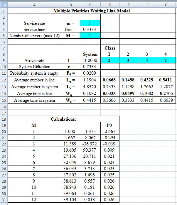
Excel Workings:
Hence the average wait time for service by customers for class 1 is 0.0333 hours, class 2 is 0.0499 hours, class 3 is 0.1082 hours and class 4 is 0.2705 hours. The waiting in each class on average for class 1 is 0.0666 customers, class 2 is 0.1498 customers, class 3 is 0.4329 customers and class 4 is 0.5411 customers.
d)
To determine: The observations based on the results from part c.
Answer to Problem 16P
Explanation of Solution
Calculate the change in average wait time for each class.
It is calculated by subtracting the final answer for average wait time for service by customers from part b with the final answer for average wait time for service by customers from part c.
Change in Average TimeClass 1=[0.3333−0.3333]=0 hours
Change in Average TimeClass 2=[0.0555−0.0499]=0.0056 hours
Change in Average TimeClass 3=[0.1202−0.1082]=0.0120 hours
Change in Average TimeClass 3=[0.2705−0.2705]=0 hours
The above results suggest that there is a decrease in average wait time for class 2 and class 3. Class 1 and 4 remains constant.
Calculate the change in average number waiting for each class.
It is calculated by subtracting the final answer for waiting on average from part b with the final answer for waiting on average from part c.
Change in Average WaitingClass 1=[0.3333−0.3333]=0 customers
Change in Average TimeClass 2=[0.2220−0.1498]=0.0722 customers
Change in Average TimeClass 3=[0.4329−0.3607]=0.0722 customers
Change in Average TimeClass 4=[0.5411−0.5411]=0 customers
The above results suggest that there is a decrease in average waiting for class 2 and an increase in class 3. Class 1 and 4 remains constant.
Want to see more full solutions like this?
Chapter 18 Solutions
EBK OPERATIONS MANAGEMENT


- The Importance of Food Labeling and Expiration Dates in a nursing home kitchen and how can a nutritionist utilize this in their career? Please not just a short explanation.arrow_forwarda) Huurhun Printing in Ulaanbaatar has four typesetters and four jobs to be completed as given in the table. The $ entries represent the firm’s estimate of what it will cost for each job to be completed by each typesetter. Find the optimal assignment of jobs to typesetters so as to minimize the total costs. Typesetters Jobs A B C D 42HG $7 $3 $4 $8 19DT $5 $4 $6 $5 47ST $6 $7 $9 $6 17VT $8 $6 $7 $4 b) Huurhun Printing in Ulaanbaatar has the following printing jobs waiting to be processed at its work center. The jobs are assigned sequentially upon arrival. All dates are specified as days from today. In what sequence should the firm process the jobs according to the SPT, EDD, and CR scheduling rules? Jobs Due Date Duration (days) 42HG 43 10 19DT 37 12 47ST 34 11 17VT 32 7 LR99 37 15arrow_forward1) Scheduling at Washburn Guitar View the video Scheduling at Washburn Guitar (10.40 minutes, Ctrl+Click on the link); what are your key takeaways (tie to one or more of the topics discussed in Chapters 11 and/or 16) after watching this video. Note: As a rough guideline, please try to keep the written submission to one or two paragraphs. 2) Bosa Limited, a specialist confectionary manufacturer, makes a variety of confectionary products candies in its manufacturing facility at Ulaanbaatar. Its line of confectionary products exhibits a highly seasonal demand pattern. The firm’s costs and quarterly sales forecasts are as follows: Costs: Hiring cost = $200 per worker, Firing cost = $600 per worker, Inventory carrying cost = $0.60 per pound per worker, Production per employee = 1000 pounds per quarter, Beginning workforce = 125 workers. Quarter Sales Forecast/ Demand(pounds) Production Spring 80,000 95,000 Summer 50,000 95,000 Fall 100,000 95,000…arrow_forward
- Note: In chapter 11, section 11.3 of the Stevenson text, level and chase plans are covered with examples (example 1, and example 2); chapter 11 Stevenson lecture power point slides 23 to 32 cover chase and level plans with an example; see lecture video, 12.21 mins to 26.55 mins. 3) a) Huurhun Printing in Ulaanbaatar has four typesetters and four jobs to be completed as given in the table. The $ entries represent the firm’s estimate of what it will cost for each job to be completed by each typesetter. Find the optimal assignment of jobs to typesetters so as to minimize the total costs. Typesetters Jobs A B C D 42HG $7 $3 $4 $8 19DT $5 $4 $6 $5 47ST $6 $7 $9 $6 17VT $8 $6 $7 $4 b) Huurhun Printing in Ulaanbaatar has the following printing jobs waiting to be processed at its work center. The jobs are assigned sequentially upon arrival. All dates are specified as days from today. In what sequence should the…arrow_forwardGalaxy Co. sells virtual reality (VR) goggles, particularly targeting customers who like to play video games. Galaxy procures each pair of goggles for $150 from its supplier and sells each pair of goggles for $300. Monthly demand for the VR goggles is a normal random variable with a mean of 157 units and a standard deviation of 41 units. At the beginning of each month, Galaxy orders enough goggles from its supplier to bring the inventory level up to 140 goggles. If the monthly demand is less than 140, Galaxy pays $20 per pair of goggles that remains in inventory at the end of the month. If the monthly demand exceeds 140, Galaxy sells only the 140 pairs of goggles in stock. Galaxy assigns a shortage cost of $40 for each unit of demand that is unsatisfied to represent a loss-of-goodwill among its customers. Management would like to use a simulation model to analyze this situation. (Use at least 1,000 trials.) (a) What is the average monthly profit (in dollars)? (Round your answer to the…arrow_forwardHospital administrators must schedule nurses so that the hospital's patients are provided adequate care. At the same time, careful attention must be paid to keeping costs down. From historical records, administrators can project the minimum number of nurses required to be on hand for various times of day and days of the week. The objective is to find the minimum total number of nurses required to provide adequate care. Nurses start work at the beginning of one of the four-hour shifts given below (except for shift 6) and work for 8 consecutive hours. Hence, possible start times are the start of shifts 1 through 5. Also, assume that the projected required number of nurses factors in time for each nurse to have a meal break. Formulate and solve the nurse scheduling problem as an integer program for one day for the data given below. (Let x = number of nurses who start work at the beginning of shift t, t = 1, 2, 3, 4, 5.) Shift Time Minimum Number of Nurses Needed 1 12:00 A.M. - 4:00 A.M.…arrow_forward
- The Kolkmeyer Manufacturing Company uses a group of six identical machines, each of which operates an average of 23 hours between breakdowns. With randomly occurring breakdowns, the Poisson probability distribution is used to describe the machine breakdown arrival process. One person from the maintenance department provides the single-server repair service for the six machines. Management is now considering adding two machines to its manufacturing operation. This addition will bring the number of machines to eight. The president of Kolkmeyer asked for a study of the need to add a second employee to the repair operation. The service rate for each individual assigned to the repair operation is 0.40 machines per hour. (a) Compute the operating characteristics if the company retains the single-employee repair operation. (Round your answers to four decimal places. Report time in hours.) W L = q W = ✓ X h × h (b) Compute the operating characteristics if a second employee is added to the…arrow_forwardConsider the nonlinear optimization model stated below. Min 2x²-18x + 2XY + y² 14Y + 51 s.t. X + 4Y ≤7 (a) Find the minimum solution to this problem. at (X, Y) = (b) If the right-hand side of the constraint is increased from 7 to 8, how much do you expect the objective function to change? Based on the dual value on the constraint X + 4Y ≤7, we expect the optimal objective function value to decrease by (c) Resolve the problem with a new right-hand side of the constraint of 8. How does the actual change compare with your estimate? If we resolve the problem with a new right-hand-side of 8 the new optimal objective function value is , so the actual change is a decrease of rather than what we expected in part (b).arrow_forwardBurger Dome sells hamburgers, cheeseburgers, french fries, soft drinks, and milk shakes, as well as a limited number of specialty items and dessert selections. Although Burger Dome would like to serve each customer immediately, at times more customers arrive than can be handled by the Burger Dome food service staff. Thus, customers wait in line to place and receive their orders. Burger Dome analyzed data on customer arrivals and concluded that the arrival rate is 40 customers per hour. Burger Dome also studied the order-filling process and found that a single employee can process an average of 56 customer orders per hour. Burger Dome is concerned that the methods currently used to serve customers are resulting in excessive waiting times and a possible loss of sales. Management wants to conduct a waiting line study to help determine the best approach to reduce waiting times and improve service. Suppose Burger Dome establishes two servers but arranges the restaurant layout so that an…arrow_forward
- >>>> e 自 A ? ↑ G סוי - C Mind Tap Cengage Learning CENGAGE MINDTAP Chapter 12 Homework: Managing Inventories in Supply Chains Assignment: Chapter 12 Homework: Managing Inventories in Supply Chains Questions Problem 12-70 Algo (Managing Fixed-Quantity Inventory Systems) 6. 7. ng.cengage.com + O C Excel Online Student Work Q Search this course ? Save Assignment Score: 91.34% Submit Assignment for Grading e Question 8 of 11 ▸ A-Z Hint(s) Check My Work 8. 9. 10. 11. Spreadsheet Environmental considerations, material losses, and waste disposal can be included in the EOQ model to improve inventory-management decisions. Assume that the annual demand for an industrial chemical is 1,600 lb, item cost is $2/lb, order cost is $45, inventory holding cost rate (percent of item cost) is 15 percent. Use the EOQ Model Excel template in MindTap to answer the following: a. Find the EOQ and total cost, assuming no waste disposal. Do not round intermediate calculations. Round your answer for the EOQ to…arrow_forward>>>> G סוי - C Mind Tap Cengage Learning CENGAGE MINDTAP Chapter 12 Homework: Managing Inventories in Supply Chains Questions Problem 12-44 Algo (Managing Fixed-Quantity Inventory Systems) 1. e 2. 3. 自 4. 5. ? ↑ 6. 7. 8. 9. 10. 11. ng.cengage.com + O C Excel Online Student Work Q Search this course ? Question 3 of 11 ► Hint(s) Check My Work Brenda opened a pool and spa store in a lively shopping mall and finds business to be booming but she often stocks out of key items customers want. The 28-ounce bottle of Super Algaecide (SA) is a high margin SKU, but it stocks out frequently. Ten SA bottles come in each box, and she orders boxes from a vendor 160 miles away. Brenda is busy running the store and seldom has time to review store inventory status and order the right quantity at the right time. She collected the following data: Demand = 9 boxes per week Order cost = $90/order Store open = 48 weeks/year Lead-time = 3 weeks Item cost = $180/box Inventory-holding cost = 10 percent per…arrow_forwardווח CENGAGE MINDTAP G Chapter 09 Excel Activity: Exponential Smoothing Question 1 3.33/10 A e Submit 自 ? G→ Video Excel Online Tutorial Excel Online Activity: Exponential Smoothing ng.cengage.com Q Search this course ? A retail store records customer demand during each sales period. The data has been collected in the Microsoft Excel Online file below. Use the Microsoft Excel Online file below to develop the single exponential smoothing forecast and answer the following questions. X Open spreadsheet Questions 1. What is the forecast for the 13th period based on the single exponential smoothing? Round your answer to two decimal places. 91.01 2. What is the MSE for the single exponential smoothing forecast? Round your answer to two decimal places. 23.50 3. Choose the correct graph for the single exponential smoothing forecast. The correct graph is graph A ☑ Back Observation Exponential Smoothing Forecast 100 Forecast 95 95 90 90 A-Z Office Next A+arrow_forward
 Practical Management ScienceOperations ManagementISBN:9781337406659Author:WINSTON, Wayne L.Publisher:Cengage,
 MarketingMarketingISBN:9780357033791Author:Pride, William MPublisher:South Western Educational Publishing