Videos
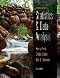
The paper referenced in Exercise 15.5 described an experiment to determine it restrictive age labeling on video games increased the attractiveness of the game for boys age 12 to 13. In that exercise, the null hypothesis
- a. Calculate the 95% T-K intervals and then use the underscoring procedure described in this section to identify significant differences among the age labels.
- b. Based on your answer to Part (a), write a few sentences commenting on the theory that the more restrictive the age label on a video game, the more attractive the game is to 12- to 13-year-old boys.

Trending nowThis is a popular solution!

Chapter 15 Solutions
Bundle: Introduction to Statistics and Data Analysis, 5th + WebAssign Printed Access Card: Peck/Olsen/Devore. 5th Edition, Single-Term


- You may need to use the appropriate appendix table or technology to answer this question. You are given the following information obtained from a random sample of 4 observations. 24 48 31 57 You want to determine whether or not the mean of the population from which this sample was taken is significantly different from 49. (Assume the population is normally distributed.) (a) State the null and the alternative hypotheses. (Enter != for ≠ as needed.) H0: Ha: (b) Determine the test statistic. (Round your answer to three decimal places.) (c) Determine the p-value, and at the 5% level of significance, test to determine whether or not the mean of the population is significantly different from 49. Find the p-value. (Round your answer to four decimal places.) p-value = State your conclusion. Reject H0. There is insufficient evidence to conclude that the mean of the population is different from 49.Do not reject H0. There is sufficient evidence to conclude that the…arrow_forward65% of all violent felons in the prison system are repeat offenders. If 43 violent felons are randomly selected, find the probability that a. Exactly 28 of them are repeat offenders. b. At most 28 of them are repeat offenders. c. At least 28 of them are repeat offenders. d. Between 22 and 26 (including 22 and 26) of them are repeat offenders.arrow_forward08:34 ◄ Classroom 07:59 Probs. 5-32/33 D ا. 89 5-34. Determine the horizontal and vertical components of reaction at the pin A and the normal force at the smooth peg B on the member. A 0,4 m 0.4 m Prob. 5-34 F=600 N fr th ar 0. 163586 5-37. The wooden plank resting between the buildings deflects slightly when it supports the 50-kg boy. This deflection causes a triangular distribution of load at its ends. having maximum intensities of w, and wg. Determine w and wg. each measured in N/m. when the boy is standing 3 m from one end as shown. Neglect the mass of the plank. 0.45 m 3 marrow_forward
- Examine the Variables: Carefully review and note the names of all variables in the dataset. Examples of these variables include: Mileage (mpg) Number of Cylinders (cyl) Displacement (disp) Horsepower (hp) Research: Google to understand these variables. Statistical Analysis: Select mpg variable, and perform the following statistical tests. Once you are done with these tests using mpg variable, repeat the same with hp Mean Median First Quartile (Q1) Second Quartile (Q2) Third Quartile (Q3) Fourth Quartile (Q4) 10th Percentile 70th Percentile Skewness Kurtosis Document Your Results: In RStudio: Before running each statistical test, provide a heading in the format shown at the bottom. “# Mean of mileage – Your name’s command” In Microsoft Word: Once you've completed all tests, take a screenshot of your results in RStudio and paste it into a Microsoft Word document. Make sure that snapshots are very clear. You will need multiple snapshots. Also transfer these results to the…arrow_forwardExamine the Variables: Carefully review and note the names of all variables in the dataset. Examples of these variables include: Mileage (mpg) Number of Cylinders (cyl) Displacement (disp) Horsepower (hp) Research: Google to understand these variables. Statistical Analysis: Select mpg variable, and perform the following statistical tests. Once you are done with these tests using mpg variable, repeat the same with hp Mean Median First Quartile (Q1) Second Quartile (Q2) Third Quartile (Q3) Fourth Quartile (Q4) 10th Percentile 70th Percentile Skewness Kurtosis Document Your Results: In RStudio: Before running each statistical test, provide a heading in the format shown at the bottom. “# Mean of mileage – Your name’s command” In Microsoft Word: Once you've completed all tests, take a screenshot of your results in RStudio and paste it into a Microsoft Word document. Make sure that snapshots are very clear. You will need multiple snapshots. Also transfer these results to the…arrow_forwardExamine the Variables: Carefully review and note the names of all variables in the dataset. Examples of these variables include: Mileage (mpg) Number of Cylinders (cyl) Displacement (disp) Horsepower (hp) Research: Google to understand these variables. Statistical Analysis: Select mpg variable, and perform the following statistical tests. Once you are done with these tests using mpg variable, repeat the same with hp Mean Median First Quartile (Q1) Second Quartile (Q2) Third Quartile (Q3) Fourth Quartile (Q4) 10th Percentile 70th Percentile Skewness Kurtosis Document Your Results: In RStudio: Before running each statistical test, provide a heading in the format shown at the bottom. “# Mean of mileage – Your name’s command” In Microsoft Word: Once you've completed all tests, take a screenshot of your results in RStudio and paste it into a Microsoft Word document. Make sure that snapshots are very clear. You will need multiple snapshots. Also transfer these results to the…arrow_forward
- 2 (VaR and ES) Suppose X1 are independent. Prove that ~ Unif[-0.5, 0.5] and X2 VaRa (X1X2) < VaRa(X1) + VaRa (X2). ~ Unif[-0.5, 0.5]arrow_forward8 (Correlation and Diversification) Assume we have two stocks, A and B, show that a particular combination of the two stocks produce a risk-free portfolio when the correlation between the return of A and B is -1.arrow_forward9 (Portfolio allocation) Suppose R₁ and R2 are returns of 2 assets and with expected return and variance respectively r₁ and 72 and variance-covariance σ2, 0%½ and σ12. Find −∞ ≤ w ≤ ∞ such that the portfolio wR₁ + (1 - w) R₂ has the smallest risk.arrow_forward
- 7 (Multivariate random variable) Suppose X, €1, €2, €3 are IID N(0, 1) and Y2 Y₁ = 0.2 0.8X + €1, Y₂ = 0.3 +0.7X+ €2, Y3 = 0.2 + 0.9X + €3. = (In models like this, X is called the common factors of Y₁, Y₂, Y3.) Y = (Y1, Y2, Y3). (a) Find E(Y) and cov(Y). (b) What can you observe from cov(Y). Writearrow_forward1 (VaR and ES) Suppose X ~ f(x) with 1+x, if 0> x > −1 f(x) = 1−x if 1 x > 0 Find VaRo.05 (X) and ES0.05 (X).arrow_forwardJoy is making Christmas gifts. She has 6 1/12 feet of yarn and will need 4 1/4 to complete our project. How much yarn will she have left over compute this solution in two different ways arrow_forward
 Holt Mcdougal Larson Pre-algebra: Student Edition...AlgebraISBN:9780547587776Author:HOLT MCDOUGALPublisher:HOLT MCDOUGAL
 Glencoe Algebra 1, Student Edition, 9780079039897...AlgebraISBN:9780079039897Author:CarterPublisher:McGraw Hill
 Big Ideas Math A Bridge To Success Algebra 1: Stu...AlgebraISBN:9781680331141Author:HOUGHTON MIFFLIN HARCOURTPublisher:Houghton Mifflin Harcourt