Concept explainers
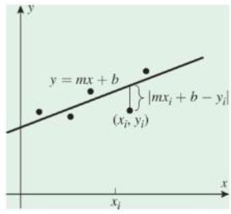
A common problem in experimental work is to obtain a mathematical relationship

These vertical distances arc called the residuals of the data points, so the effect of minimizing
The purpose of this exercise is to find the values of m and b that produce the regression line.
(a) To minimize
(b) Let
(c) Assuming that not all the
[Note: We have shown that g has a critical point at these values of m and b. In the next exercise we will show that g has an absolute minimum at this critical point. Accepting this to be so, we have shown that the line
Want to see the full answer?
Check out a sample textbook solution
Chapter 13 Solutions
Calculus Early Transcendentals, Binder Ready Version
Additional Math Textbook Solutions
Algebra and Trigonometry (6th Edition)
Probability And Statistical Inference (10th Edition)
Introductory Statistics
Elementary Statistics (13th Edition)
College Algebra (7th Edition)
Pre-Algebra Student Edition
- Consider the graphs of y = f(x) and y = g(x) in the given diagram y= f(x). y = g(x) Evaluate (f+g)(2) -5 Determine all for which g(x) < f(x) Determine all for which f(x) +3 = g(x)arrow_forwardI) For what value(s) of x does g(x) = -4? Separate multiple answers with commas as needed. J) Give the interval(s) of such that g(x) > 0. Use the union symbol between multiple intervals. K) Give the interval(s) of such that g(x) <0. Use the union symbol between multiple intervals.arrow_forwardneed help on Barrow_forward
- 4. Use the properties of limits to help decide whether each limit exists. If a limit exists, fi lim (2x²-4x+5) a) x-4 b) lim 2 x²-16 x-4x+2x-8arrow_forward7. The concentration of a drug in a patient's bloodstream h hours after it was injected is given by 0.17 h Ah= h²+2' Find and interpret lim A(h). Remember, the answers to word problems should always be given in a complete h→00 sentence, with proper units, in the context of the problem.arrow_forward#2arrow_forward
- 2. We want to find the inverse of f(x) = (x+3)² a. On the graph at right, sketch f(x). (Hint: use what you know about transformations!) (2 points) b. What domain should we choose to get only the part of f (x) that is one- to-one and non-decreasing? Give your answer in inequality notation. (2 points) - c. Now use algebra to find f¯¹ (x). (2 points) -4- 3- 2 1 -4 -3 -2 -1 0 1 -1- -2- --3- -4 -N- 2 3 4arrow_forward1. Suppose f(x) = 2 4 == x+3 and g(x) = ½-½. Find and fully simplify ƒ(g(x)). Be sure to show all x your work, write neatly so your work is easy to follow, and connect your expressions with equals signs. (4 points)arrow_forwardFind the ane sided limit lim 2 x+1-3x-3arrow_forward
- Algebra & Trigonometry with Analytic GeometryAlgebraISBN:9781133382119Author:SwokowskiPublisher:Cengage
