a. To state:
The null and alternative hypothesis.
Answer to Problem 18E
Solution:
The null hypothesis is
Explanation of Solution
Consider the following scenario,
“Teachers’ salaries in one state are very low, so low that educators in that state regularly complain about their compensation. The state
State the null and alternative hypothesis.
Suppose teachers claims that mean in their district is significantly lower than state mean of $33, 600. That is the research hypothesis mathematically as
The Null hypothesis:
The alternative hypothesis:
Final statement:
The null hypothesis is
b. To determine:
Which distribution to use for the test statistic, and state the level of significance.
Answer to Problem 18E
Solution:
The t-test statistic is used and the level of significance of
Explanation of Solution
The t-test statistic is appropriate to use in this case because the claim is about a population mean, the populations
So, t-test statistic is used and the level of significance of
Final statement:
The t-test statistic is used and the level of significance of
c. To gather:
The data and calculate the necessary sample statistics.
Answer to Problem 18E
Solution:
The calculated test statistic is -3.7030.
Explanation of Solution
The test statistic formula:
Test statistic for a hypothesis test for a population mean (
When the population standard deviation is unknown, the sample taken is a simple random sample, and either the sample size is at least 30 or the population distribution is approximately normal, the test statistic for a hypothesis test for a population mean is given by,
Where n is the sample size,
The given information is,
Substitute these values in the test statistic formula to get the following,
So, the calculated test statistic is -3.7030.
Final statement:
The calculated test statistic is -3.7030.
d. To draw:
To Draw a conclusion and interpret the decision.
Answer to Problem 18E
Solution:
There is a significance evidence to support the teachers’ claims that the mean in their district is significantly lower at the 0.01 level of significance.
Explanation of Solution
Assume that the population standard deviation is unknown and the population distribution is approximately normal.
Rejection Region for Hypothesis Tests for Population Means (
If p-value
If p- value
Degrees of Freedom for t in a Hypothesis Test for a Population Means (
In a hypothesis test for a population mean where the population standard deviation is unknown, the number of degrees of freedom for the Student’s t- distribution of the test statistic is given by
Where n is the sample size.
Form the given information this is the left-tailed test since
From the given information n = 22 then the degrees of freedom is given below,
Conclusion:
Consider the level of significance of
Use the “p value of t-test statistic” calculator to get the following,
The p -value is approximately 0.0007. Since
The diagrammatic representation is given below,
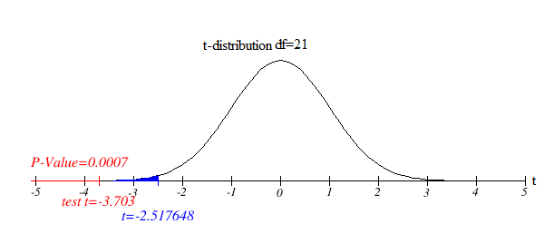
Thus the conclusion is to reject the null hypothesis.
So, there is significance evidence to support the teachers’ claims that the mean in their district is significantly lower at the 0.01 level of significance.
Final statement:
There is a significance evidence to support the teachers’ claims that the mean in their district is significantly lower at the 0.01 level of significance.
Want to see more full solutions like this?
Chapter 10 Solutions
Beginning Statistics, 2nd Edition

- A marketing agency wants to determine whether different advertising platforms generate significantly different levels of customer engagement. The agency measures the average number of daily clicks on ads for three platforms: Social Media, Search Engines, and Email Campaigns. The agency collects data on daily clicks for each platform over a 10-day period and wants to test whether there is a statistically significant difference in the mean number of daily clicks among these platforms. Conduct ANOVA test. You can provide your answer by inserting a text box and the answer must include: also please provide a step by on getting the answers in excel Null hypothesis, Alternative hypothesis, Show answer (output table/summary table), and Conclusion based on the P value.arrow_forwardA company found that the daily sales revenue of its flagship product follows a normal distribution with a mean of $4500 and a standard deviation of $450. The company defines a "high-sales day" that is, any day with sales exceeding $4800. please provide a step by step on how to get the answers Q: What percentage of days can the company expect to have "high-sales days" or sales greater than $4800? Q: What is the sales revenue threshold for the bottom 10% of days? (please note that 10% refers to the probability/area under bell curve towards the lower tail of bell curve) Provide answers in the yellow cellsarrow_forwardBusiness Discussarrow_forward
- The following data represent total ventilation measured in liters of air per minute per square meter of body area for two independent (and randomly chosen) samples. Analyze these data using the appropriate non-parametric hypothesis testarrow_forwardeach column represents before & after measurements on the same individual. Analyze with the appropriate non-parametric hypothesis test for a paired design.arrow_forwardShould you be confident in applying your regression equation to estimate the heart rate of a python at 35°C? Why or why not?arrow_forward
 MATLAB: An Introduction with ApplicationsStatisticsISBN:9781119256830Author:Amos GilatPublisher:John Wiley & Sons Inc
 Probability and Statistics for Engineering and th...StatisticsISBN:9781305251809Author:Jay L. DevorePublisher:Cengage Learning
 Statistics for The Behavioral Sciences (MindTap C...StatisticsISBN:9781305504912Author:Frederick J Gravetter, Larry B. WallnauPublisher:Cengage Learning
 Elementary Statistics: Picturing the World (7th E...StatisticsISBN:9780134683416Author:Ron Larson, Betsy FarberPublisher:PEARSON
 The Basic Practice of StatisticsStatisticsISBN:9781319042578Author:David S. Moore, William I. Notz, Michael A. FlignerPublisher:W. H. Freeman
 Introduction to the Practice of StatisticsStatisticsISBN:9781319013387Author:David S. Moore, George P. McCabe, Bruce A. CraigPublisher:W. H. Freeman