Chapter 10.1, Problem 34E

Solution

a)

The value of r2 and the fit of least square line in the data.

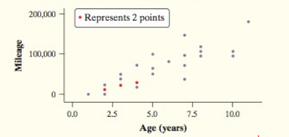
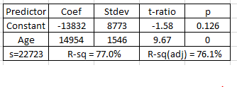
Given:The dot plot and Minitab output for least squares regression analysis for these data.

  

  

Explanation:

From the Minitab output, the value of R-sq is 77%. This is interpreted as 77% of variation in the mileage is explained by the linear relationship with age (in years) of cars.

b)

The mean mileage of the cars in the sample where mean age is 8 years.

The mean mileage for the sample is 105,800 miles.

Given:The regression line equation

  $\hat{y}=-13,832+14954x$

Calculation:

The regression line equation pass through the point mean of age and mean of mileage $\left(\stackrel{\_\_}{x},\stackrel{\_\_}{y}\right)$

plug in the value of mean age in the regression line equation we get

  $\begin{array}{l}\hat{y}=-13,832+14954x\\ \stackrel{\_\_}{y}=-13,832+14954\stackrel{\_\_}{x}\\ \stackrel{\_\_}{y}=-13832+14954*8=105800\end{array}$

Conclusion:the mean mileage of the cars in the sample is 105,800 miles when the car is 8 years old on an average.

c)

Interpret the value of standard deviation in this context.

Given:

The standard deviation from Minitab output is 22723.

Explanation:

The least square regression line is used to predict the mileage of cars using its age. Here the standard deviation of the residuals (s) gives the approximation of prediction error. So on average a difference of 22723 miles between the actual mileage and predicted mileage.

d)

Is it reasonable to use the least squares line to predict a cars mileage from its age for a Council high school teacher?

Explanation:

Here the data given and Minitab output are used to predict the mileage of cars owned by students using its age. Since the least square line is based on sample of cars owned by students not teachers, it is not reasonable to use the least squares line to predict a car’s mileage from its age for a teacher.