Videos
For Problems 7-21, please provide the following information.
(a) What is the level of significance? Stale the null and alternate hypotheses, (b) Check Requirements What sampling distribution will you use? Do you think the sample size is sufficiently large? Explain Compute the value of the sample test statistic and corresponding z value. (c) Find the P-value of the test statistic Sketch the sampling distribution and show the area corresponding to the P-value.
(d) Based on sour answers in parts (a) to (c), will you reject or fail to reject the null hypothesis? Are the data statistic ally significant at level a?
(c) Interpret your conclusion in the context of the application.
Focus Problem: Benford's Law Again, suppose you are the auditor for a very large corporation. The revenue file contains millions of numbers in a large computer data bank (see Problem 7). You draw a random sample of n = 228 numbers from this file, and r = 92 have a first nonzero digit of 1.
Let p represent the population proportion of all numbers in the computer file that have a leading digit of 1.
i.Test the claim that p is more than 0.301. Use
ii.If p is in fact larger than 0.301, it would seem there are too many numbers in the file with leading 1s. Could this indicate that the books have been “cooked" by artificially lowering numbers in the file? Comment from the point of view of the Internal Revenue Service, Comment from the perspective of the Federal Bureau of Investigation as it looks for "profit skimming" by unscrupulous employees.
iii.Comment on the following statement: "If we reject the null hypothesis at level of significance
(i)
(a)
The level of significance, null and alternative hypothesis.
Answer to Problem 8P
Solution: The level of significance is
Explanation of Solution
The level of significance is defined as the probability of rejecting the null hypothesis when it is true, it is denoted by
Null hypothesis
Alternative hypothesis
(b)
To find: The sampling distribution that should be used and compute the z value of the sample test statistic.
Answer to Problem 8P
Solution: The sampling distribution
Explanation of Solution
Calculation:
The
The standardized sample test statistic for
(c)
To find: The P-value of the test statistic and sketch the sampling distribution showing the area corresponding to the P-value.
Answer to Problem 8P
Solution: The P-value of the test statistic is 0.0004.
Explanation of Solution
Calculation:
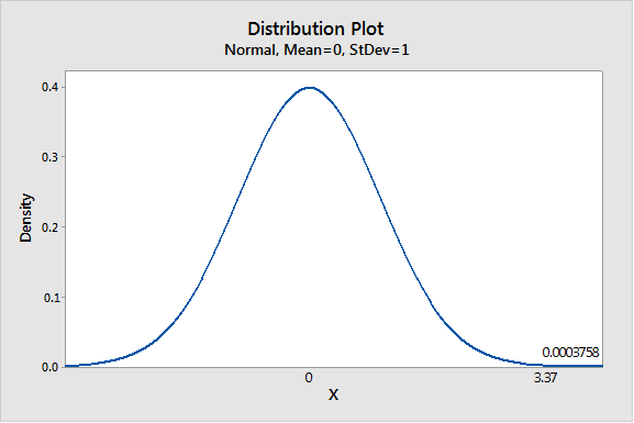
We have z = 3.37
Using Table 3 from the Appendix to find the specified area:
Thus P- value is 0.0004.
Graph:
To draw the required graphs using the Minitab, follow the below instructions:
Step 1: Go to the Minitab software.
Step 2: Go to Graph > Probability distribution plot > View probability.
Step 3: Select ‘Normal’ and enter Mean 0 and Standard deviation 1.
Step 4: Click on the Shaded area > X value.
Step 5: Enter X-value as 3.37 and select ‘Right tail’.
Step 6: Click on OK.
The obtained distribution graph is:
(d)
Whether we reject or fail to reject the null hypothesisand whether the data is statistically significant for a level of significance of 0.01.
Answer to Problem 8P
Solution: The P-value
Explanation of Solution
The P-value of 0.0004 is less than the level of significance (
(e)
The interpretation for the conclusion.
Answer to Problem 8P
Solution: There is sufficient evidence to conclude that population proportion of numbers with leading “1” in the revenue file is more than the probability 0.301.
Explanation of Solution
The P-value of 0.0004 is less than the level of significance (
(ii)
To explain: Whether it is suspect that there are too many numbers in the data file with leading 1's.
Answer to Problem 8P
Solution: Yes. The revenue data file seems to be too many entries with leading digit 1.
Explanation of Solution
There are too many numbers in the data file with leading 1's. So, we cannot say that it is an indication of the books have been “cooked” by artificially lowering numbers in the file. From the viewpoint of the Internal Revenue Service and the Federal Bureau of Investigation as it looks for “profit skimming”, it may be true or false because there are too many numbers in the data file with leading 1’s.
(iii)
To explain: Whether it recommends further investigation before accusing the company of fraud.
Answer to Problem 8P
Solution: Our data lead us to reject the null hypothesis, more investigation is merited.
Explanation of Solution
Since, we reject the null hypothesis
Want to see more full solutions like this?
Chapter 9 Solutions
Bundle: Understanding Basic Statistics, Loose-leaf Version, 7th + WebAssign Printed Access Card for Brase/Brase's Understanding Basic Statistics, ... for Peck's Statistics: Learning from Data


- Examine the Variables: Carefully review and note the names of all variables in the dataset. Examples of these variables include: Mileage (mpg) Number of Cylinders (cyl) Displacement (disp) Horsepower (hp) Research: Google to understand these variables. Statistical Analysis: Select mpg variable, and perform the following statistical tests. Once you are done with these tests using mpg variable, repeat the same with hp Mean Median First Quartile (Q1) Second Quartile (Q2) Third Quartile (Q3) Fourth Quartile (Q4) 10th Percentile 70th Percentile Skewness Kurtosis Document Your Results: In RStudio: Before running each statistical test, provide a heading in the format shown at the bottom. “# Mean of mileage – Your name’s command” In Microsoft Word: Once you've completed all tests, take a screenshot of your results in RStudio and paste it into a Microsoft Word document. Make sure that snapshots are very clear. You will need multiple snapshots. Also transfer these results to the…arrow_forwardExamine the Variables: Carefully review and note the names of all variables in the dataset. Examples of these variables include: Mileage (mpg) Number of Cylinders (cyl) Displacement (disp) Horsepower (hp) Research: Google to understand these variables. Statistical Analysis: Select mpg variable, and perform the following statistical tests. Once you are done with these tests using mpg variable, repeat the same with hp Mean Median First Quartile (Q1) Second Quartile (Q2) Third Quartile (Q3) Fourth Quartile (Q4) 10th Percentile 70th Percentile Skewness Kurtosis Document Your Results: In RStudio: Before running each statistical test, provide a heading in the format shown at the bottom. “# Mean of mileage – Your name’s command” In Microsoft Word: Once you've completed all tests, take a screenshot of your results in RStudio and paste it into a Microsoft Word document. Make sure that snapshots are very clear. You will need multiple snapshots. Also transfer these results to the…arrow_forwardExamine the Variables: Carefully review and note the names of all variables in the dataset. Examples of these variables include: Mileage (mpg) Number of Cylinders (cyl) Displacement (disp) Horsepower (hp) Research: Google to understand these variables. Statistical Analysis: Select mpg variable, and perform the following statistical tests. Once you are done with these tests using mpg variable, repeat the same with hp Mean Median First Quartile (Q1) Second Quartile (Q2) Third Quartile (Q3) Fourth Quartile (Q4) 10th Percentile 70th Percentile Skewness Kurtosis Document Your Results: In RStudio: Before running each statistical test, provide a heading in the format shown at the bottom. “# Mean of mileage – Your name’s command” In Microsoft Word: Once you've completed all tests, take a screenshot of your results in RStudio and paste it into a Microsoft Word document. Make sure that snapshots are very clear. You will need multiple snapshots. Also transfer these results to the…arrow_forward
- 2 (VaR and ES) Suppose X1 are independent. Prove that ~ Unif[-0.5, 0.5] and X2 VaRa (X1X2) < VaRa(X1) + VaRa (X2). ~ Unif[-0.5, 0.5]arrow_forward8 (Correlation and Diversification) Assume we have two stocks, A and B, show that a particular combination of the two stocks produce a risk-free portfolio when the correlation between the return of A and B is -1.arrow_forward9 (Portfolio allocation) Suppose R₁ and R2 are returns of 2 assets and with expected return and variance respectively r₁ and 72 and variance-covariance σ2, 0%½ and σ12. Find −∞ ≤ w ≤ ∞ such that the portfolio wR₁ + (1 - w) R₂ has the smallest risk.arrow_forward
- 7 (Multivariate random variable) Suppose X, €1, €2, €3 are IID N(0, 1) and Y2 Y₁ = 0.2 0.8X + €1, Y₂ = 0.3 +0.7X+ €2, Y3 = 0.2 + 0.9X + €3. = (In models like this, X is called the common factors of Y₁, Y₂, Y3.) Y = (Y1, Y2, Y3). (a) Find E(Y) and cov(Y). (b) What can you observe from cov(Y). Writearrow_forward1 (VaR and ES) Suppose X ~ f(x) with 1+x, if 0> x > −1 f(x) = 1−x if 1 x > 0 Find VaRo.05 (X) and ES0.05 (X).arrow_forwardJoy is making Christmas gifts. She has 6 1/12 feet of yarn and will need 4 1/4 to complete our project. How much yarn will she have left over compute this solution in two different ways arrow_forward
- Solve for X. Explain each step. 2^2x • 2^-4=8arrow_forwardOne hundred people were surveyed, and one question pertained to their educational background. The results of this question and their genders are given in the following table. Female (F) Male (F′) Total College degree (D) 30 20 50 No college degree (D′) 30 20 50 Total 60 40 100 If a person is selected at random from those surveyed, find the probability of each of the following events.1. The person is female or has a college degree. Answer: equation editor Equation Editor 2. The person is male or does not have a college degree. Answer: equation editor Equation Editor 3. The person is female or does not have a college degree.arrow_forwardneed help with part barrow_forward
 College Algebra (MindTap Course List)AlgebraISBN:9781305652231Author:R. David Gustafson, Jeff HughesPublisher:Cengage Learning
 Glencoe Algebra 1, Student Edition, 9780079039897...AlgebraISBN:9780079039897Author:CarterPublisher:McGraw Hill