Concept explainers
Videos
Please provide the following information for Problems 11-22.
(a) What is the level of significance? State the null and alternate hypotheses.
(b)Check Requirements What sampling distribution will you use? Explain the rationale for your choice of sampling distribution. Compute the appropriate sampling distribution value of the sample test statistic.
(c) Find (or estimate) the P-value. Sketch the sampling distribution and show the area corresponding to the P- value.
(d) Based on your answers in parts (a) to (c), will you reject or fail to reject the null hypothesis? Are the data statistically significant at level ?
(e)Interpret your conclusion in the context of the application.
Note: For degrees of freedom d.f. not given in the Student's t table, use the closest d.f. that is smaller. In some situations, this choice of d.f. may increase the P-value by a small amount and therefore produce a slightly more “conservative" answer.
Fishing: Atlantic Salmon Homser Lake. Oregon, has an Atlantic salmon catch and release program that has been very successful. The average fisherman's catch has been
| 12 | 6 | 11 | 12 | 5 | 0 | 2 |
| 7 | 8 | 7 | 6 | 3 | 12 | 12 |
Use a calculator with
ii.Assuming the catch per day has an approximately
(i)
Whether the sample mean
Answer to Problem 21P
Solution: Yes, the sample mean
Explanation of Solution
To calculate the required statistics using the Minitab, follow the below instructions:
Step 1: Go to the Minitab software.
Step 2: Go to Stat > Basic statistics > Display Descriptive Statistics.
Step 3: Select ‘Catches’ in variables.
Step 4: Click on OK.
The obtained statistics is:
Descriptive Statistics: Catches
Statistics
| Variable | N | N* | Mean | SE Mean | StDev | Minimum | Q1 | Median | Q3 | Maximum |
| Catches | 14 | 0 | 7.36 | 1.08 | 4.03 | 0.00 | 4.50 | 7.00 | 12.00 | 12.00 |
From the Minitab output, the sample mean and sample standard deviation are approximately equals to
(ii)
(a)
The level of significance, null and alternative hypothesis.
Answer to Problem 21P
Solution: The level of significance is
Explanation of Solution
The level of significance is defined as the probability of rejecting the null hypothesis when it is true, it is denoted by
Null hypothesis
Alternative hypothesis
(b)
To find: The sampling distribution that should be used and compute the value of the sample test statistic.
Answer to Problem 21P
Solution: The student’s t distribution should be used. The sample test statistic is -1.34.
Explanation of Solution
Calculation:
We assume that x distribution is mound shape and symmetrical, because
Using
The sample test statistic t is
(c)
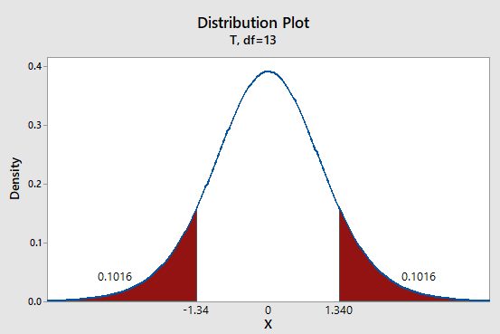
To find: The P-value of the test statistic and sketch the sampling distribution showing the area corresponding to the P-value.
Answer to Problem 21P
Solution: The P-value of the test statistic is 0.2032.
Explanation of Solution
Calculation:
We have t = -1.34
Using Table 4 from the Appendix to find the specified area:
Graph:
To draw the required graphs using the Minitab, follow the below instructions:
Step 1: Go to the Minitab software.
Step 2: Go to Graph > Probability distribution plot > View probability.
Step 3: Select ‘t’ and enter d.f = 13.
Step 4: Click on the Shaded area >X value.
Step 5: Enter X-value as -1.34 and select ‘Both Tail’.
Step 6: Click on OK.
The obtained distribution graph is:
(d)
Whether we reject or fail to reject the null hypothesis and whether the data is statistically significant for a level of significance of 0.05.
Answer to Problem 21P
Solution: The P-value
Explanation of Solution
The P-value of 0.2032 is greater than the level of significance (
) of 0.05. Therefore we don’t have enough evidence to reject the null hypothesis
(e)
The interpretation for the conclusion.
Answer to Problem 21P
Solution: There is not enough evidence to conclude that population average catch per day is now different from 8.8.
Explanation of Solution
The P-value of 0.2032 is greater than the level of significance (
) of 0.05. Therefore we don’t have enough evidence to reject the null hypothesis
Want to see more full solutions like this?
Chapter 9 Solutions
Bundle: Understanding Basic Statistics, Loose-leaf Version, 7th + WebAssign Printed Access Card for Brase/Brase's Understanding Basic Statistics, ... for Peck's Statistics: Learning from Data


- 3. (i) Consider the following R code: wilcox.test(UK Supermarkets $Salary ~ UKSupermarkets $Supermarket) (a) Which test is being used in this code? (b) What is the name of the dataset under consideration? How would be adapt this code if we had ties? What other command can be used which deals with ties? (ii) Consider the following R code: install packages("nortest") library(nortest) lillie.test (Differences) (a) Assuming the appropriate dataset has been imported and attached, what is wrong with this code? (b) If this code were to be corrected, what would be determined by run- ning it? [3 Marks]arrow_forward1. (i) Explain the difference in application between the Mann-Whitney U test and the Wilcoxon Signed-Rank test, i.e. in which scenarios would each test be used? (ii) What is the main procedure underlying these nonparametric tests? [3 Marks]arrow_forwardYou may need to use the appropriate appendix table or technology to answer this question. You are given the following information obtained from a random sample of 4 observations. 24 48 31 57 You want to determine whether or not the mean of the population from which this sample was taken is significantly different from 49. (Assume the population is normally distributed.) (a) State the null and the alternative hypotheses. (Enter != for ≠ as needed.) H0: Ha: (b) Determine the test statistic. (Round your answer to three decimal places.) (c) Determine the p-value, and at the 5% level of significance, test to determine whether or not the mean of the population is significantly different from 49. Find the p-value. (Round your answer to four decimal places.) p-value = State your conclusion. Reject H0. There is insufficient evidence to conclude that the mean of the population is different from 49.Do not reject H0. There is sufficient evidence to conclude that the…arrow_forward
- 65% of all violent felons in the prison system are repeat offenders. If 43 violent felons are randomly selected, find the probability that a. Exactly 28 of them are repeat offenders. b. At most 28 of them are repeat offenders. c. At least 28 of them are repeat offenders. d. Between 22 and 26 (including 22 and 26) of them are repeat offenders.arrow_forward08:34 ◄ Classroom 07:59 Probs. 5-32/33 D ا. 89 5-34. Determine the horizontal and vertical components of reaction at the pin A and the normal force at the smooth peg B on the member. A 0,4 m 0.4 m Prob. 5-34 F=600 N fr th ar 0. 163586 5-37. The wooden plank resting between the buildings deflects slightly when it supports the 50-kg boy. This deflection causes a triangular distribution of load at its ends. having maximum intensities of w, and wg. Determine w and wg. each measured in N/m. when the boy is standing 3 m from one end as shown. Neglect the mass of the plank. 0.45 m 3 marrow_forwardExamine the Variables: Carefully review and note the names of all variables in the dataset. Examples of these variables include: Mileage (mpg) Number of Cylinders (cyl) Displacement (disp) Horsepower (hp) Research: Google to understand these variables. Statistical Analysis: Select mpg variable, and perform the following statistical tests. Once you are done with these tests using mpg variable, repeat the same with hp Mean Median First Quartile (Q1) Second Quartile (Q2) Third Quartile (Q3) Fourth Quartile (Q4) 10th Percentile 70th Percentile Skewness Kurtosis Document Your Results: In RStudio: Before running each statistical test, provide a heading in the format shown at the bottom. “# Mean of mileage – Your name’s command” In Microsoft Word: Once you've completed all tests, take a screenshot of your results in RStudio and paste it into a Microsoft Word document. Make sure that snapshots are very clear. You will need multiple snapshots. Also transfer these results to the…arrow_forward
- Examine the Variables: Carefully review and note the names of all variables in the dataset. Examples of these variables include: Mileage (mpg) Number of Cylinders (cyl) Displacement (disp) Horsepower (hp) Research: Google to understand these variables. Statistical Analysis: Select mpg variable, and perform the following statistical tests. Once you are done with these tests using mpg variable, repeat the same with hp Mean Median First Quartile (Q1) Second Quartile (Q2) Third Quartile (Q3) Fourth Quartile (Q4) 10th Percentile 70th Percentile Skewness Kurtosis Document Your Results: In RStudio: Before running each statistical test, provide a heading in the format shown at the bottom. “# Mean of mileage – Your name’s command” In Microsoft Word: Once you've completed all tests, take a screenshot of your results in RStudio and paste it into a Microsoft Word document. Make sure that snapshots are very clear. You will need multiple snapshots. Also transfer these results to the…arrow_forwardExamine the Variables: Carefully review and note the names of all variables in the dataset. Examples of these variables include: Mileage (mpg) Number of Cylinders (cyl) Displacement (disp) Horsepower (hp) Research: Google to understand these variables. Statistical Analysis: Select mpg variable, and perform the following statistical tests. Once you are done with these tests using mpg variable, repeat the same with hp Mean Median First Quartile (Q1) Second Quartile (Q2) Third Quartile (Q3) Fourth Quartile (Q4) 10th Percentile 70th Percentile Skewness Kurtosis Document Your Results: In RStudio: Before running each statistical test, provide a heading in the format shown at the bottom. “# Mean of mileage – Your name’s command” In Microsoft Word: Once you've completed all tests, take a screenshot of your results in RStudio and paste it into a Microsoft Word document. Make sure that snapshots are very clear. You will need multiple snapshots. Also transfer these results to the…arrow_forward2 (VaR and ES) Suppose X1 are independent. Prove that ~ Unif[-0.5, 0.5] and X2 VaRa (X1X2) < VaRa(X1) + VaRa (X2). ~ Unif[-0.5, 0.5]arrow_forward
- 8 (Correlation and Diversification) Assume we have two stocks, A and B, show that a particular combination of the two stocks produce a risk-free portfolio when the correlation between the return of A and B is -1.arrow_forward9 (Portfolio allocation) Suppose R₁ and R2 are returns of 2 assets and with expected return and variance respectively r₁ and 72 and variance-covariance σ2, 0%½ and σ12. Find −∞ ≤ w ≤ ∞ such that the portfolio wR₁ + (1 - w) R₂ has the smallest risk.arrow_forward7 (Multivariate random variable) Suppose X, €1, €2, €3 are IID N(0, 1) and Y2 Y₁ = 0.2 0.8X + €1, Y₂ = 0.3 +0.7X+ €2, Y3 = 0.2 + 0.9X + €3. = (In models like this, X is called the common factors of Y₁, Y₂, Y3.) Y = (Y1, Y2, Y3). (a) Find E(Y) and cov(Y). (b) What can you observe from cov(Y). Writearrow_forward
 Glencoe Algebra 1, Student Edition, 9780079039897...AlgebraISBN:9780079039897Author:CarterPublisher:McGraw Hill
 College Algebra (MindTap Course List)AlgebraISBN:9781305652231Author:R. David Gustafson, Jeff HughesPublisher:Cengage Learning
 Holt Mcdougal Larson Pre-algebra: Student Edition...AlgebraISBN:9780547587776Author:HOLT MCDOUGALPublisher:HOLT MCDOUGAL