Concept explainers
Videos
(a)
Verify the values of
(a)
Explanation of Solution
Calculation:
The variable x denotes a random variable that represents the percentage of successful free throws a professional basketball player makes in a season and y denotes a random variable that represents the percentage of successful field goals a professional basketball player makes in a season.
The formula for
In the formula, n is the
The values are verified in the table below,
| x | y | xy | ||
| 67 | 44 | 4489 | 1936 | 2948 |
| 65 | 42 | 4225 | 1764 | 2730 |
| 75 | 48 | 5625 | 2304 | 3600 |
| 86 | 51 | 7396 | 2601 | 4386 |
| 73 | 44 | 5329 | 1936 | 3212 |
| 73 | 51 | 5329 | 2601 | 3723 |
Hence, the values are verified.
The number of data pairs are
Hence, the value of r is verified as approximately 0.784.
(b)
Check whether the claim
(b)
Answer to Problem 7P
The claim
Explanation of Solution
Calculation:
Null hypothesis:
Alternative hypothesis:
Test statistic:
The test statistic formula for test
Where r is the sample correlation coefficient, n is the sample size with degrees of freedom
Substitute r as 0.784, and n as 6 in the test statistic formula.
The test statistic value is 2.526.
The degrees of freedom is,
Step by step procedure to obtain P-value using MINITAB software is given below:
- Choose Graph > Probability Distribution Plot choose View Probability > OK.
- From Distribution, choose ‘t’ distribution.
- Enter the Degrees of freedom as 4.
- Click the Shaded Area tab.
- Choose X Value and Right Tail, for the region of the curve to shade.
- Enter the X value as 2.526.
- Click OK.
Output using MINITAB software is given below:
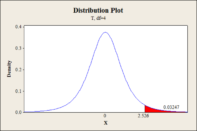
From Minitab output, the P-value is 0.0325.
Rejection rule:
- If the P-value is less than or equal to
Conclusion:
The P-value is 0.0325 and the level of significance is 0.05.
The P-value is less than the level of significance.
That is,
By the rejection rule, the null hypothesis is rejected.
Hence, the claim
(c)
Verify the values of
(c)
Explanation of Solution
Calculation:
The value of
The value of
The value of
The value of
The value of b is,
The value of b is 0.4117.
The value of a is,
The value of a is 16.542.
The value of
The value of
The equation of the least-squares line is,
The regression equation is
(d)
Find the predicted percentage
(d)
Answer to Problem 7P
The predicted percentage
Explanation of Solution
Calculation:
The regression equation is
Substitute x as 70 in the regression equation
Hence, the predicted percentage
(e)
Find the 90% confidence interval for y when
(e)
Answer to Problem 7P
The 90% confidence interval for y when
Explanation of Solution
Calculation:
Step by step procedure to obtain confidence interval using MINITAB software is given below:
- Choose Stat > Regression > Regression.
- In Response, enter the column containing the response as y.
- In Predictors, enter the columns containing the predictor as x.
- Choose Options.
- In Prediction intervals for new observations, enter the value as 70.
- In Confidence level, enter value as 90.
- Click OK.
Output using MINITAB software is given below:
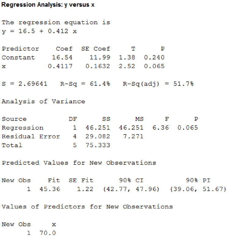
From Minitab output, the confidence interval is
Hence, the 90% confidence interval for y when
(f)
Check whether the claim
(f)
Answer to Problem 7P
The claim
Explanation of Solution
Calculation:
Null hypothesis:
Alternative hypothesis:
Test statistic:
The test statistic formula for slope
Where
Substitute
The test statistic value is 2.522.
The degrees of freedom is,
Step by step procedure to obtain P-value using MINITAB software is given below:
- Choose Graph > Probability Distribution Plot choose View Probability > OK.
- From Distribution, choose ‘t’ distribution.
- Enter the Degrees of freedom as 4.
- Click the Shaded Area tab.
- Choose X Value and Right Tail, for the region of the curve to shade.
- Enter the X value as 2.522.
- Click OK.
Output using MINITAB software is given below:

From Minitab output, the P-value is 0.0326.
Rejection rule:
- If the P-value is less than or equal to
Conclusion:
The P-value is 0.0326 and the level of significance is 0.05.
The P-value is less than the level of significance.
That is,
By the rejection rule, the null hypothesis is rejected.
Hence, the claim
(g)
Find a 90% confidence interval for
Interpret the confidence interval.
(g)
Answer to Problem 7P
The 90% confidence interval for
Explanation of Solution
Calculation:
Confidence interval for slope:
The confidence interval formula for slope
Where
Critical value:
Use the Appendix II: Tables, Table 6: Critical Values for Student’s t Distribution:
- In d.f. column locate the value 4.
- In the row of two-tail area locate the level of significance
- The intersecting value of row and columns is 2.132.
The critical value is
The margin of error is,
The 90% confidence interval for
Hence, the 90% confidence interval for
The percentage of successful field goals for a basketball player increases by an amount that ranges between 0.064 and 0.760, if percentage of successful free throws increases by one unit.
Want to see more full solutions like this?
Chapter 9 Solutions
Bundle: Understandable Statistics, Loose-leaf Version, 12th + WebAssign Printed Access Card for Brase/Brase's Understandable Statistics: Concepts and Methods, 12th Edition, Single-Term


- High Cholesterol: A group of eight individuals with high cholesterol levels were given a new drug that was designed to lower cholesterol levels. Cholesterol levels, in milligrams per deciliter, were measured before and after treatment for each individual, with the following results: Individual Before 1 2 3 4 5 6 7 8 237 282 278 297 243 228 298 269 After 200 208 178 212 174 201 189 185 Part: 0/2 Part 1 of 2 (a) Construct a 99.9% confidence interval for the mean reduction in cholesterol level. Let a represent the cholesterol level before treatment minus the cholesterol level after. Use tables to find the critical value and round the answers to at least one decimal place.arrow_forwardI worked out the answers for most of this, and provided the answers in the tables that follow. But for the total cost table, I need help working out the values for 10%, 11%, and 12%. A pharmaceutical company produces the drug NasaMist from four chemicals. Today, the company must produce 1000 pounds of the drug. The three active ingredients in NasaMist are A, B, and C. By weight, at least 8% of NasaMist must consist of A, at least 4% of B, and at least 2% of C. The cost per pound of each chemical and the amount of each active ingredient in one pound of each chemical are given in the data at the bottom. It is necessary that at least 100 pounds of chemical 2 and at least 450 pounds of chemical 3 be used. a. Determine the cheapest way of producing today’s batch of NasaMist. If needed, round your answers to one decimal digit. Production plan Weight (lbs) Chemical 1 257.1 Chemical 2 100 Chemical 3 450 Chemical 4 192.9 b. Use SolverTable to see how much the percentage of…arrow_forwardAt the beginning of year 1, you have $10,000. Investments A and B are available; their cash flows per dollars invested are shown in the table below. Assume that any money not invested in A or B earns interest at an annual rate of 2%. a. What is the maximized amount of cash on hand at the beginning of year 4.$ ___________ A B Time 0 -$1.00 $0.00 Time 1 $0.20 -$1.00 Time 2 $1.50 $0.00 Time 3 $0.00 $1.90arrow_forward
- For each of the time series, construct a line chart of the data and identify the characteristics of the time series (that is, random, stationary, trend, seasonal, or cyclical). Year Month Rate (%)2009 Mar 8.72009 Apr 9.02009 May 9.42009 Jun 9.52009 Jul 9.52009 Aug 9.62009 Sep 9.82009 Oct 10.02009 Nov 9.92009 Dec 9.92010 Jan 9.82010 Feb 9.82010 Mar 9.92010 Apr 9.92010 May 9.62010 Jun 9.42010 Jul 9.52010 Aug 9.52010 Sep 9.52010 Oct 9.52010 Nov 9.82010 Dec 9.32011 Jan 9.12011 Feb 9.02011 Mar 8.92011 Apr 9.02011 May 9.02011 Jun 9.12011 Jul 9.02011 Aug 9.02011 Sep 9.02011 Oct 8.92011 Nov 8.62011 Dec 8.52012 Jan 8.32012 Feb 8.32012 Mar 8.22012 Apr 8.12012 May 8.22012 Jun 8.22012 Jul 8.22012 Aug 8.12012 Sep 7.82012 Oct…arrow_forwardFor each of the time series, construct a line chart of the data and identify the characteristics of the time series (that is, random, stationary, trend, seasonal, or cyclical). Date IBM9/7/2010 $125.959/8/2010 $126.089/9/2010 $126.369/10/2010 $127.999/13/2010 $129.619/14/2010 $128.859/15/2010 $129.439/16/2010 $129.679/17/2010 $130.199/20/2010 $131.79 a. Construct a line chart of the closing stock prices data. Choose the correct chart below.arrow_forwardFor each of the time series, construct a line chart of the data and identify the characteristics of the time series (that is, random, stationary, trend, seasonal, or cyclical) Date IBM9/7/2010 $125.959/8/2010 $126.089/9/2010 $126.369/10/2010 $127.999/13/2010 $129.619/14/2010 $128.859/15/2010 $129.439/16/2010 $129.679/17/2010 $130.199/20/2010 $131.79arrow_forward
- 1. A consumer group claims that the mean annual consumption of cheddar cheese by a person in the United States is at most 10.3 pounds. A random sample of 100 people in the United States has a mean annual cheddar cheese consumption of 9.9 pounds. Assume the population standard deviation is 2.1 pounds. At a = 0.05, can you reject the claim? (Adapted from U.S. Department of Agriculture) State the hypotheses: Calculate the test statistic: Calculate the P-value: Conclusion (reject or fail to reject Ho): 2. The CEO of a manufacturing facility claims that the mean workday of the company's assembly line employees is less than 8.5 hours. A random sample of 25 of the company's assembly line employees has a mean workday of 8.2 hours. Assume the population standard deviation is 0.5 hour and the population is normally distributed. At a = 0.01, test the CEO's claim. State the hypotheses: Calculate the test statistic: Calculate the P-value: Conclusion (reject or fail to reject Ho): Statisticsarrow_forward21. find the mean. and variance of the following: Ⓒ x(t) = Ut +V, and V indepriv. s.t U.VN NL0, 63). X(t) = t² + Ut +V, U and V incepires have N (0,8) Ut ①xt = e UNN (0162) ~ X+ = UCOSTE, UNNL0, 62) SU, Oct ⑤Xt= 7 where U. Vindp.rus +> ½ have NL, 62). ⑥Xn = ΣY, 41, 42, 43, ... Yn vandom sample K=1 Text with mean zen and variance 6arrow_forwardA psychology researcher conducted a Chi-Square Test of Independence to examine whether there is a relationship between college students’ year in school (Freshman, Sophomore, Junior, Senior) and their preferred coping strategy for academic stress (Problem-Focused, Emotion-Focused, Avoidance). The test yielded the following result: image.png Interpret the results of this analysis. In your response, clearly explain: Whether the result is statistically significant and why. What this means about the relationship between year in school and coping strategy. What the researcher should conclude based on these findings.arrow_forward
- A school counselor is conducting a research study to examine whether there is a relationship between the number of times teenagers report vaping per week and their academic performance, measured by GPA. The counselor collects data from a sample of high school students. Write the null and alternative hypotheses for this study. Clearly state your hypotheses in terms of the correlation between vaping frequency and academic performance. EditViewInsertFormatToolsTable 12pt Paragrapharrow_forwardA smallish urn contains 25 small plastic bunnies – 7 of which are pink and 18 of which are white. 10 bunnies are drawn from the urn at random with replacement, and X is the number of pink bunnies that are drawn. (a) P(X = 5) ≈ (b) P(X<6) ≈ The Whoville small urn contains 100 marbles – 60 blue and 40 orange. The Grinch sneaks in one night and grabs a simple random sample (without replacement) of 15 marbles. (a) The probability that the Grinch gets exactly 6 blue marbles is [ Select ] ["≈ 0.054", "≈ 0.043", "≈ 0.061"] . (b) The probability that the Grinch gets at least 7 blue marbles is [ Select ] ["≈ 0.922", "≈ 0.905", "≈ 0.893"] . (c) The probability that the Grinch gets between 8 and 12 blue marbles (inclusive) is [ Select ] ["≈ 0.801", "≈ 0.760", "≈ 0.786"] . The Whoville small urn contains 100 marbles – 60 blue and 40 orange. The Grinch sneaks in one night and grabs a simple random sample (without replacement) of 15 marbles. (a)…arrow_forwardSuppose an experiment was conducted to compare the mileage(km) per litre obtained by competing brands of petrol I,II,III. Three new Mazda, three new Toyota and three new Nissan cars were available for experimentation. During the experiment the cars would operate under same conditions in order to eliminate the effect of external variables on the distance travelled per litre on the assigned brand of petrol. The data is given as below: Brands of Petrol Mazda Toyota Nissan I 10.6 12.0 11.0 II 9.0 15.0 12.0 III 12.0 17.4 13.0 (a) Test at the 5% level of significance whether there are signi cant differences among the brands of fuels and also among the cars. [10] (b) Compute the standard error for comparing any two fuel brands means. Hence compare, at the 5% level of significance, each of fuel brands II, and III with the standard fuel brand I. [10] �arrow_forward
 Glencoe Algebra 1, Student Edition, 9780079039897...AlgebraISBN:9780079039897Author:CarterPublisher:McGraw Hill