Concept explainers
Videos
(a)
Construct a
Verify the values of
Find the value of r.
(a)
Answer to Problem 23P
The scatter diagram for data is,
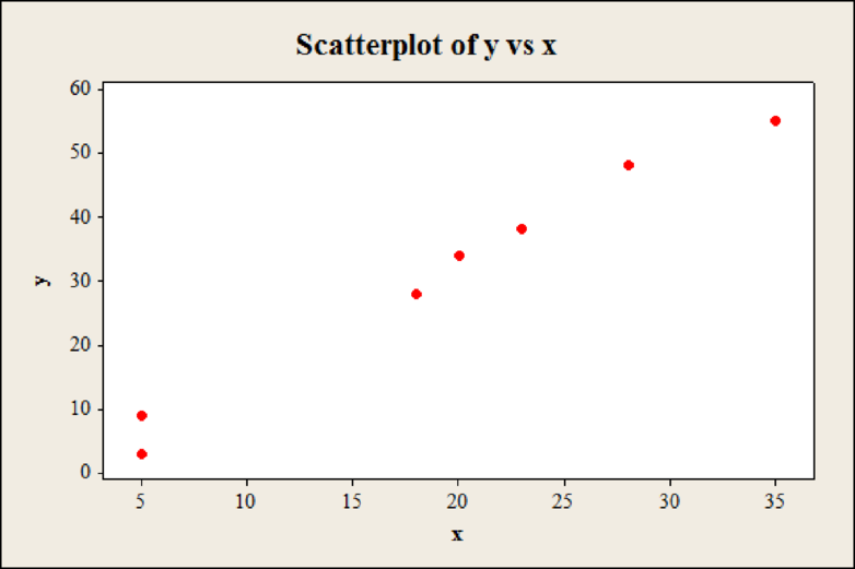
The value of r is 0.991.
Explanation of Solution
Calculation:
The formula for
In the formula, n is the sample size.
The variable x denotes average annual hours per person spent in traffic delays and y denotes the average annual gallons of fuel wasted per person in traffic delays.
Step by step procedure to obtain scatter plot using MINITAB software is given below:
- Choose Graph > Scatterplot.
- Choose Simple. Click OK.
- In Y variables, enter the column of x.
- In X variables, enter the column of y.
- Click OK.
The values are verified in the table below,
| x | y | xy | ||
| 28 | 48 | 784 | 2304 | 1344 |
| 5 | 3 | 25 | 9 | 15 |
| 20 | 34 | 400 | 1156 | 680 |
| 35 | 55 | 1225 | 3025 | 1925 |
| 20 | 34 | 400 | 1156 | 680 |
| 23 | 38 | 529 | 1444 | 874 |
| 18 | 28 | 324 | 784 | 504 |
| 5 | 9 | 25 | 81 | 45 |
Hence, the values are verified.
The number of data pairs are
Hence, the value of r is 0.991.
(b)
Find the value of
Find the value of
Find the value of
Find the value of
Identify the set in which standard deviations for x and y is larger.
Explain why standard deviations increase the value of r.
(b)
Answer to Problem 23P
The value of
The value of
The value of
The value of
The value of
The value of
The value of
The value of
The standard deviation for variables based on single individuals is larger.
The values of
Explanation of Solution
Calculation:
Mean and standard deviation for variables based on averages:
Step by step procedure to obtain mean and standard deviation using MINITAB software is given as,
- Choose Stat > Basic Statistics > Display
Descriptive Statistics . - In Variables enter the column x, y.
- Choose option statistics, and select Mean, standard deviation.
- Click OK.
Output using MINITAB software is given below:
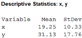
From MINITAB output, the mean of x is 19.25, the mean of y is 31.13, and standard deviation of x is 10.33, the standard deviation of y is 17.76.
Hence, the value of
Mean and standard deviation for variables based on single individuals:
Step by step procedure to obtain mean and standard deviation using MINITAB software is given as,
- Choose Stat > Basic Statistics > Display Descriptive Statistics.
- In Variables enter the column x, y.
- Choose option statistics, and select Mean, standard deviation.
- Click OK.
Output using MINITAB software is given below:
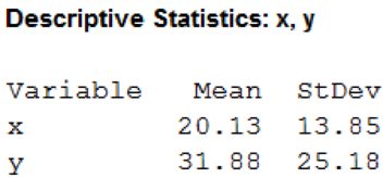
From MINITAB output, the mean of x is 20.13, the mean of y is 31.88, and standard deviation of x is 13.85, the standard deviation of y is 25.18.
Hence, the value of
It can be observed that value of
The formula for correlation coefficient r in equation (1) is,
In the formula the values of
(c)
Construct a scatter diagram for the second set of data.
Verify the values of
Find the value of r.
(c)
Answer to Problem 23P
The scatter diagram for second set of data is,
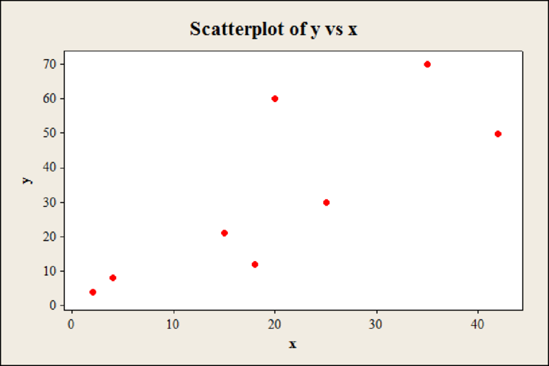
The value of r is 0.794.
Explanation of Solution
Calculation:
The variable x denotes average annual number of hours lost for the person and y denotes the average annual gallons of fuel wasted for the person.
Step by step procedure to obtain scatter plot using MINITAB software is given below:
- Choose Graph > Scatterplot.
- Choose Simple. Click OK.
- In Y variables, enter the column of x.
- In X variables, enter the column of y.
- Click OK.
The values are verified in the table below,
| x | y | xy | ||
| 20 | 60 | 400 | 3600 | 1200 |
| 4 | 8 | 16 | 64 | 32 |
| 18 | 12 | 324 | 144 | 216 |
| 42 | 50 | 1764 | 2500 | 2100 |
| 15 | 21 | 225 | 441 | 315 |
| 25 | 30 | 625 | 900 | 750 |
| 2 | 4 | 4 | 16 | 8 |
| 35 | 70 | 1225 | 4900 | 2450 |
Hence, the values are verified.
The number of data pairs are
Hence, the value of r is 0.794.
(d)
Identify the data for averages have a higher
Mention the reasons why hours lost per individual and fuel wasted per individual might vary more than the same quantities averaged over all the people in a city.
(d)
Explanation of Solution
From part (a), the value of r for averages is 0.991. From part (c), the value of r for single observations is 0.794.
It can be observed that, the correlation coefficient for data of averages is larger than correlation coefficient for data of single observations.
The values of standard deviations for variables x and y based on data of averages are smaller when compared to the values of standard deviations for variables x and y based on data of single observations. The smaller standard deviation results in larger value of r, giving a higher correlation coefficient for data of averages.
Also, based on the central limit theorem the distribution of x distribution has the larger standard deviation when compared to
Want to see more full solutions like this?
Chapter 9 Solutions
Bundle: Understandable Statistics, Loose-leaf Version, 12th + WebAssign Printed Access Card for Brase/Brase's Understandable Statistics: Concepts and Methods, 12th Edition, Single-Term


- II Consider the following data matrix X: X1 X2 0.5 0.4 0.2 0.5 0.5 0.5 10.3 10 10.1 10.4 10.1 10.5 What will the resulting clusters be when using the k-Means method with k = 2. In your own words, explain why this result is indeed expected, i.e. why this clustering minimises the ESS map.arrow_forwardwhy the answer is 3 and 10?arrow_forwardPS 9 Two films are shown on screen A and screen B at a cinema each evening. The numbers of people viewing the films on 12 consecutive evenings are shown in the back-to-back stem-and-leaf diagram. Screen A (12) Screen B (12) 8 037 34 7 6 4 0 534 74 1645678 92 71689 Key: 116|4 represents 61 viewers for A and 64 viewers for B A second stem-and-leaf diagram (with rows of the same width as the previous diagram) is drawn showing the total number of people viewing films at the cinema on each of these 12 evenings. Find the least and greatest possible number of rows that this second diagram could have. TIP On the evening when 30 people viewed films on screen A, there could have been as few as 37 or as many as 79 people viewing films on screen B.arrow_forward
- Q.2.4 There are twelve (12) teams participating in a pub quiz. What is the probability of correctly predicting the top three teams at the end of the competition, in the correct order? Give your final answer as a fraction in its simplest form.arrow_forwardThe table below indicates the number of years of experience of a sample of employees who work on a particular production line and the corresponding number of units of a good that each employee produced last month. Years of Experience (x) Number of Goods (y) 11 63 5 57 1 48 4 54 5 45 3 51 Q.1.1 By completing the table below and then applying the relevant formulae, determine the line of best fit for this bivariate data set. Do NOT change the units for the variables. X y X2 xy Ex= Ey= EX2 EXY= Q.1.2 Estimate the number of units of the good that would have been produced last month by an employee with 8 years of experience. Q.1.3 Using your calculator, determine the coefficient of correlation for the data set. Interpret your answer. Q.1.4 Compute the coefficient of determination for the data set. Interpret your answer.arrow_forwardCan you answer this question for mearrow_forward
- Techniques QUAT6221 2025 PT B... TM Tabudi Maphoru Activities Assessments Class Progress lIE Library • Help v The table below shows the prices (R) and quantities (kg) of rice, meat and potatoes items bought during 2013 and 2014: 2013 2014 P1Qo PoQo Q1Po P1Q1 Price Ро Quantity Qo Price P1 Quantity Q1 Rice 7 80 6 70 480 560 490 420 Meat 30 50 35 60 1 750 1 500 1 800 2 100 Potatoes 3 100 3 100 300 300 300 300 TOTAL 40 230 44 230 2 530 2 360 2 590 2 820 Instructions: 1 Corall dawn to tha bottom of thir ceraan urina se se tha haca nariad in archerca antarand cubmit Q Search ENG US 口X 2025/05arrow_forwardThe table below indicates the number of years of experience of a sample of employees who work on a particular production line and the corresponding number of units of a good that each employee produced last month. Years of Experience (x) Number of Goods (y) 11 63 5 57 1 48 4 54 45 3 51 Q.1.1 By completing the table below and then applying the relevant formulae, determine the line of best fit for this bivariate data set. Do NOT change the units for the variables. X y X2 xy Ex= Ey= EX2 EXY= Q.1.2 Estimate the number of units of the good that would have been produced last month by an employee with 8 years of experience. Q.1.3 Using your calculator, determine the coefficient of correlation for the data set. Interpret your answer. Q.1.4 Compute the coefficient of determination for the data set. Interpret your answer.arrow_forwardQ.3.2 A sample of consumers was asked to name their favourite fruit. The results regarding the popularity of the different fruits are given in the following table. Type of Fruit Number of Consumers Banana 25 Apple 20 Orange 5 TOTAL 50 Draw a bar chart to graphically illustrate the results given in the table.arrow_forward
- Q.2.3 The probability that a randomly selected employee of Company Z is female is 0.75. The probability that an employee of the same company works in the Production department, given that the employee is female, is 0.25. What is the probability that a randomly selected employee of the company will be female and will work in the Production department? Q.2.4 There are twelve (12) teams participating in a pub quiz. What is the probability of correctly predicting the top three teams at the end of the competition, in the correct order? Give your final answer as a fraction in its simplest form.arrow_forwardQ.2.1 A bag contains 13 red and 9 green marbles. You are asked to select two (2) marbles from the bag. The first marble selected will not be placed back into the bag. Q.2.1.1 Construct a probability tree to indicate the various possible outcomes and their probabilities (as fractions). Q.2.1.2 What is the probability that the two selected marbles will be the same colour? Q.2.2 The following contingency table gives the results of a sample survey of South African male and female respondents with regard to their preferred brand of sports watch: PREFERRED BRAND OF SPORTS WATCH Samsung Apple Garmin TOTAL No. of Females 30 100 40 170 No. of Males 75 125 80 280 TOTAL 105 225 120 450 Q.2.2.1 What is the probability of randomly selecting a respondent from the sample who prefers Garmin? Q.2.2.2 What is the probability of randomly selecting a respondent from the sample who is not female? Q.2.2.3 What is the probability of randomly…arrow_forwardTest the claim that a student's pulse rate is different when taking a quiz than attending a regular class. The mean pulse rate difference is 2.7 with 10 students. Use a significance level of 0.005. Pulse rate difference(Quiz - Lecture) 2 -1 5 -8 1 20 15 -4 9 -12arrow_forward
 Big Ideas Math A Bridge To Success Algebra 1: Stu...AlgebraISBN:9781680331141Author:HOUGHTON MIFFLIN HARCOURTPublisher:Houghton Mifflin Harcourt
 Glencoe Algebra 1, Student Edition, 9780079039897...AlgebraISBN:9780079039897Author:CarterPublisher:McGraw Hill
 Holt Mcdougal Larson Pre-algebra: Student Edition...AlgebraISBN:9780547587776Author:HOLT MCDOUGALPublisher:HOLT MCDOUGAL