
Concept explainers
Videos
a.
Find the value of t-test statistic.
a.
Answer to Problem 3CYU
The value of t-test statistic is 3.072787.
Explanation of Solution
Calculation:
The given statistics for testing the hypothesis
Requirements for a small sample t-test:
- The samples must be independent and drawn randomly from the populations.
- Either the sample size must be greater than 30 or the population must be approximately normal.
Here, it is given that independent random samples are drawn from approximately normal populations.
Thus, the conditions are satisfied.
The hypotheses are given below:
Null hypothesis:
Alternate hypothesis:
The test statistic for the small sample t is obtained as follows:
Under the null hypothesis,
Therefore the test statistic is,
Thus, the test statistic is 3.072787.
b.
Find the number of degrees of freedom for the test statistic.
b.
Answer to Problem 3CYU
The number of degrees of freedom for the test statistic is 9.
Explanation of Solution
Calculation:
Degrees of freedom:
The degrees of freedom for t using computer package is,
The degrees of freedom, when computing by hand is smaller of
The degrees of freedom is,
Thus, the degree of freedom is 9.
c.
Find the P-value.
c.
Answer to Problem 3CYU
The P-value is 0.006647.
Explanation of Solution
Calculation:
P-value:
Step-by-step procedure to obtain the P-value using the MINITAB software:
- Choose Graph > Probability Distribution Plot
- Choose View Probability > OK.
- From Distribution, choose ‘t’ distribution.
- In Degrees of freedom, enter 9.
- Click the Shaded Area tab.
- Choose X value and Right Tail for the region of the curve to shade.
- In X-value enter 3.072787.
- Click OK.
Output using the MINITAB software is given below:
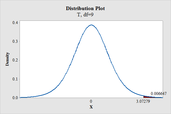
From the MINITAB output, the P-value is 0.006647.
Thus, the P-value is 0.006647.
d.
Interpret the P-value.
Check whether the null hypothesis is rejected at
d.
Answer to Problem 3CYU
There is enough evidence to reject the null hypothesis at
Explanation of Solution
Decision rule based on P-value:
If
If
Here, the level of significance is
Conclusion based on P-value approach:
The P-value is 0.006647 and
Here, P-value is less than the
That is,
By the rejection rule, reject the null hypothesis.
Hence, the null hypothesis is rejected at
Thus, it can be concluded that there is no sufficient evidence to infer the equality of two population means at
Want to see more full solutions like this?
Chapter 9 Solutions
ALEKS 360 ESSENT. STAT ACCESS CARD


- Critically analyze the following graph and, based on statistical information, indicate the type of error it presents IN NO MORE THAN 3 LINES SCOTCEN POLL OF POLLS SHOULD SCOTLAND BE INDEPENDENT? NO 52% YES 58% LIVE CAW NAS & 28.30 HAS KILLED MORE THAN 2,600 IN WEST AFRICA, WORLD HEALTH ORG. BROOKEBCNNarrow_forwardCritically analyze the following graph and, based on statistical information, indicate the type of error it presents IN NO MORE THAN 3 LINES PRESIDENTIAL PREFERENCES RODOLFO CARTER 3% (+2pts) EVELYN MATTHEI 22% (+6pts) With the exception of President Boric, could you tell me who you would like to be the next president of Chile? CAMILA VALLEJO 4% (+2pts) JOSÉ ANTONIO KAST 19% (+5pts) MICHELLE BACHELET 6% (+1pts)arrow_forwardCritically analyze the following graph and, based on statistical information, indicate the type of error it presents IN NO MORE THAN 3 LINES 13% APPROVE 4% DOESN'T KNOW DOESN'T RESPOND 5% NEITHER APPROVES NOR DISAPPROVES 78% DISAPPROVES SURVEY PRESIDENTIAL APPROVAL DROPS TO 13%arrow_forward
- Please help with this following question I'm not too sure if question (a) and (b) are correct and not sure how to calculate (c) The csv data is below "","New","Current" "1","67",66 "2","77",73 "3","76",73 "4","76",76 "5","77",79 "6","84",76 "7","71",78 "8","84",72 "9","73",76 "10","71",73 "11","72",77 "12","70",72 "13","75",72 "14","84",71 "15","77",73 "16","65",72 "17","69",73 "18","71",73 "19","79",71 "20","75",78 "21","76",69 "22","73",74 "23","76",71 "24","64",74 "25","81",78 "26","79",76 "27","70",77 "28","79",71 "29","84",73 "30","79",69 "31","69",72 "32","81",76 "33","77",70 "34","77",71 "35","71",69 "36","67",72 "37","70",76 "38","77",73 "39","82",73 "40","72",73arrow_forwardPlease help me answer the following question(c) A previous study found that 15% of nurses reported participating in mental health support programs.From the 96% found in (b) , can you conclude that proportion of nurses reported participating in mental health support programs p(current), has changed from the previous study?(Yes/No) because the confidence interval in (b) (captures/does not capture) 15%.(d) Refer to your answer in (b) : The Alberta Nurses Association expects that not more than 23 % of nurses will participate in the survey on mental health support programs. Given the result in part (b) can we conclude that this expectation is reasonable?(Yes/No) because the (upper bound/lower bound) of the 96% confidence interval is (less than/not less than/greater than) 23%. The Alberta Nursing Association conducts an annual survey to estimate the proportion of nurses who participate in mental health support programs. The most recent application of this survey involved a random sample of…arrow_forwardPlease help me solve this questionThis is what was in the csv file:"","Diabetic","Heart Disease""1",32644,30646"2",789,1670"3",12802,36274"4",2177,5011"5",1910,3300"6",3320,4256"7",61425,39053"8",19768,28635"9",19502,39546"10",5642,12182"11",107864,152098"12",29918,60433"13",2397,3550"14",41559,34705"15",49169,57948"16",72853,83100"17",2155,2873"18",140220,134517"19",28181,26212"20",18850,38637"21",69564,68582"22",13897,12613"23",6868,9138"24",9735,4767"25",12102,13447"26",36571,50010"27",44665,55141"28",26620,33970"29",25525,29766"30",14167,20206Q(b) From this, the relationship between these two variables is (non-existent/positive/negative) . I can categorize this relationship as being (strong/weak/moderate).Q(c) Drop down is (+/-)Q(d) Drop downs in order are __% of the (average/median/variation/standard deviation) in the (the number of people diagnosed with heart disease/the number of people diagnosed with diabetes)−variable can be explained by its (linear relationship/relationship)…arrow_forward
- Please help me answer the following question The drop down for question (e, f, and g) is (YES/NO) Based on the P-value above, the assumption of equal variances among the four machines (Is Met/Is Not Met) Based on the data, the average fill for machine 3 is (statistically lower than/statistically higher than/the same as/not statistically different than/statistically different than/Hard to say then when comparing to/Refuse to say when comparing to) machine 1.arrow_forwardBusiness Discussarrow_forward1 for all k, and set o (ii) Let X1, X2, that P(Xkb) = x > 0. Xn be independent random variables with mean 0, suppose = and Var Xk. Then, for 0x) ≤2 exp-tx+121 Στ k=1arrow_forward
- Lemma 1.1 Suppose that g is a non-negative, non-decreasing function such that E g(X) 0. Then, E g(|X|) P(|X|> x) ≤ g(x)arrow_forwardProof of this Theorem Theorem 1.2 (i) Suppose that P(|X| ≤ b) = 1 for some b > 0, that E X = 0, and set Var X = o². Then, for 0 0, P(X > x) ≤ e−1x+1²², P(|X|> x) ≤ 2e−x+1² 0²arrow_forwardState and prove the Morton's inequality Theorem 1.1 (Markov's inequality) Suppose that E|X|" 0, and let x > 0. Then, E|X|" P(|X|> x) ≤ x"arrow_forward
 MATLAB: An Introduction with ApplicationsStatisticsISBN:9781119256830Author:Amos GilatPublisher:John Wiley & Sons Inc
 Probability and Statistics for Engineering and th...StatisticsISBN:9781305251809Author:Jay L. DevorePublisher:Cengage Learning
 Statistics for The Behavioral Sciences (MindTap C...StatisticsISBN:9781305504912Author:Frederick J Gravetter, Larry B. WallnauPublisher:Cengage Learning
 Elementary Statistics: Picturing the World (7th E...StatisticsISBN:9780134683416Author:Ron Larson, Betsy FarberPublisher:PEARSON
 The Basic Practice of StatisticsStatisticsISBN:9781319042578Author:David S. Moore, William I. Notz, Michael A. FlignerPublisher:W. H. Freeman
 Introduction to the Practice of StatisticsStatisticsISBN:9781319013387Author:David S. Moore, George P. McCabe, Bruce A. CraigPublisher:W. H. Freeman