
Videos
The Environmental Protection Agency and the University of Florida recently cooperated in a large study of the possible effects of trace elements in drinking water on kidney-stone disease. The accompanying table presents data on age, amount of calcium in home drinking water (measured in parts per million), and smoking activity. These data were obtained from individuals with recurrent kidney-stone problems, all of whom lived in the Carolinas and the Rocky Mountain states.
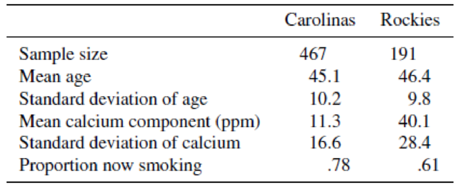
- a Estimate the average calcium concentration in drinking water for kidney-stone patients in the Carolinas. Place a bound on the error of estimation.
- b Estimate the difference in
mean ages for kidney-stone patients in the Carolinas and in the Rockies. Place a bound on the error of estimation. - c Estimate and place a 2-standard-deviation bound on the difference in proportions of kidney-stone patients from the Carolinas and Rockies who were smokers at the time of the study.
a.
Evaluate the mean calcium concentration in drinking water for kidney-stone patients in Region C.
Obtain the bound on error of estimation.
Answer to Problem 23E
The point estimate for the mean calcium concentration in drinking water for kidney-stone patients in Region C is 11.3 ppm.
The bound on the error of estimation is 1.5.
Explanation of Solution
Based on the given information, the data for calcium concentration in drinking water for kidney-stone patient in Region C is observed as given below:
The critical value has to be obtained for
Step-by-step procedure to obtain the critical value using Applet:
- Go to Applets/Simulations.
- Select Student’s t Probabilities and Quantiles.
- In df, enter 466.
- In Probability, enter 0.025.
The output obtained is as follows:
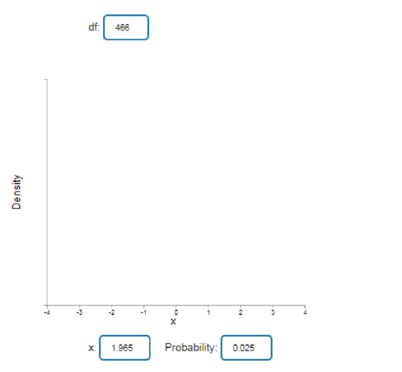
From the output, it is clear that the critical value is 1.965.
Substitute the values in two sided t-interval formula as given below:
Therefore, the point estimate for the mean calcium concentration in drinking water for kidney-stone patients in Region C is 11.3 ppm and the bound on the error of estimation is 1.5.
b.
Evaluate the difference in mean ages for kidney-stone patients in Region C and Region R.
Obtain the bound on error of estimation.
Answer to Problem 23E
The point estimate for the difference in mean ages for kidney-stone patients in Region C and Region R is −1.3
The bound on the error of estimation is 1.67.
Explanation of Solution
Based on the given information, the data are observed as given below:
Critical value:
The critical value is obtained as follows:
Step-by-step procedure to obtain the critical value using Applet:
- Go to Applets/Simulations.
- Select Student’s t Probabilities and Quantiles.
- In df, enter 656.
- In Probability, enter 0.025.
The output obtained is as follows:
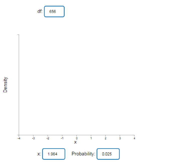
From the output, it is clear that the critical value is 1.964.
Substitute the values in two sided t-interval formula as given below:
Therefore, the point estimate for the difference in mean ages for kidney-stone patients in Region C and Region R is −1.3 and the bound on the error of estimation is 1.67.
c.
Evaluate and place 2-standard deviations bound on the difference in proportions of kidney-stone patients from Regions C and R.
Obtain the bound on error of estimation.
Answer to Problem 23E
The point estimate for the difference in proportions of kidney-stone patients from Regions C and R is 0.17, that is, (−2.97, 0.37).
The 2-standard deviations bound on the error of estimation is 0.0079.
Explanation of Solution
Based on the given information, the data are observed as given below:
The formula for difference in proportion is as follows:
Substitute the values as given below:
The point estimate for the difference in proportions of kidney-stone patients from Regions C and R is 0.17, and the 2-standard deviations bound on the error of estimation is 0.0079.
Want to see more full solutions like this?
Chapter 8 Solutions
Mathematical Statistics with Applications


- Examine the Variables: Carefully review and note the names of all variables in the dataset. Examples of these variables include: Mileage (mpg) Number of Cylinders (cyl) Displacement (disp) Horsepower (hp) Research: Google to understand these variables. Statistical Analysis: Select mpg variable, and perform the following statistical tests. Once you are done with these tests using mpg variable, repeat the same with hp Mean Median First Quartile (Q1) Second Quartile (Q2) Third Quartile (Q3) Fourth Quartile (Q4) 10th Percentile 70th Percentile Skewness Kurtosis Document Your Results: In RStudio: Before running each statistical test, provide a heading in the format shown at the bottom. “# Mean of mileage – Your name’s command” In Microsoft Word: Once you've completed all tests, take a screenshot of your results in RStudio and paste it into a Microsoft Word document. Make sure that snapshots are very clear. You will need multiple snapshots. Also transfer these results to the…arrow_forward2 (VaR and ES) Suppose X1 are independent. Prove that ~ Unif[-0.5, 0.5] and X2 VaRa (X1X2) < VaRa(X1) + VaRa (X2). ~ Unif[-0.5, 0.5]arrow_forward8 (Correlation and Diversification) Assume we have two stocks, A and B, show that a particular combination of the two stocks produce a risk-free portfolio when the correlation between the return of A and B is -1.arrow_forward
- 9 (Portfolio allocation) Suppose R₁ and R2 are returns of 2 assets and with expected return and variance respectively r₁ and 72 and variance-covariance σ2, 0%½ and σ12. Find −∞ ≤ w ≤ ∞ such that the portfolio wR₁ + (1 - w) R₂ has the smallest risk.arrow_forward7 (Multivariate random variable) Suppose X, €1, €2, €3 are IID N(0, 1) and Y2 Y₁ = 0.2 0.8X + €1, Y₂ = 0.3 +0.7X+ €2, Y3 = 0.2 + 0.9X + €3. = (In models like this, X is called the common factors of Y₁, Y₂, Y3.) Y = (Y1, Y2, Y3). (a) Find E(Y) and cov(Y). (b) What can you observe from cov(Y). Writearrow_forward1 (VaR and ES) Suppose X ~ f(x) with 1+x, if 0> x > −1 f(x) = 1−x if 1 x > 0 Find VaRo.05 (X) and ES0.05 (X).arrow_forward
- Joy is making Christmas gifts. She has 6 1/12 feet of yarn and will need 4 1/4 to complete our project. How much yarn will she have left over compute this solution in two different ways arrow_forwardSolve for X. Explain each step. 2^2x • 2^-4=8arrow_forwardOne hundred people were surveyed, and one question pertained to their educational background. The results of this question and their genders are given in the following table. Female (F) Male (F′) Total College degree (D) 30 20 50 No college degree (D′) 30 20 50 Total 60 40 100 If a person is selected at random from those surveyed, find the probability of each of the following events.1. The person is female or has a college degree. Answer: equation editor Equation Editor 2. The person is male or does not have a college degree. Answer: equation editor Equation Editor 3. The person is female or does not have a college degree.arrow_forward
 Glencoe Algebra 1, Student Edition, 9780079039897...AlgebraISBN:9780079039897Author:CarterPublisher:McGraw Hill
 Big Ideas Math A Bridge To Success Algebra 1: Stu...AlgebraISBN:9781680331141Author:HOUGHTON MIFFLIN HARCOURTPublisher:Houghton Mifflin Harcourt
 Linear Algebra: A Modern IntroductionAlgebraISBN:9781285463247Author:David PoolePublisher:Cengage Learning
 Functions and Change: A Modeling Approach to Coll...AlgebraISBN:9781337111348Author:Bruce Crauder, Benny Evans, Alan NoellPublisher:Cengage Learning