
Introduction To Statistics And Data Analysis
6th Edition
ISBN: 9781337793612
Author: PECK, Roxy.
Publisher: Cengage Learning,
expand_more
expand_more
format_list_bulleted
Concept explainers
Videos
Textbook Question
Chapter 8.1, Problem 7E
Consider the following population: {1, 2, 3, 4}. For this population the
Suppose that a random
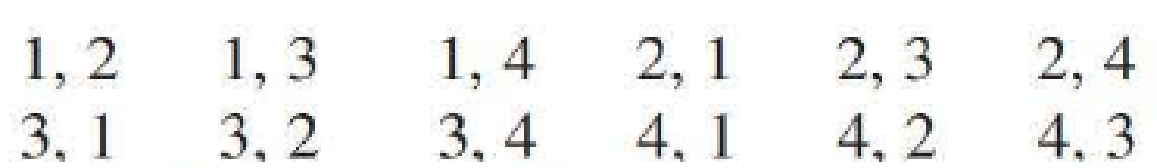
- a. Calculate the sample mean for each of the 12 possible samples.
- b. Use the sample means to construct the sampling distribution of x̄. Display the sampling distribution as a density histogram.
- c. Suppose that a random sample of size 2 is to be selected, but this time sampling will be done with replacement. Using a method similar to that of Part (a), construct the sampling distribution of x̄. (Hint: There are 16 different possible samples in this case.)
- d. In what ways are the two sampling distributions of Parts (b) and (c) similar? In what ways are they different?
Expert Solution & Answer

Trending nowThis is a popular solution!

Students have asked these similar questions
Can you answer this question for me
Techniques QUAT6221 2025 PT B...
TM
Tabudi Maphoru
Activities Assessments Class Progress lIE Library • Help v
The table below shows the prices (R) and quantities (kg) of rice, meat and potatoes items bought during 2013 and 2014:
2013
2014
P1Qo
PoQo
Q1Po P1Q1
Price
Ро
Quantity
Qo
Price
P1
Quantity
Q1
Rice
7
80
6
70
480
560
490
420
Meat
30
50
35
60
1 750
1 500
1 800
2 100
Potatoes
3
100
3
100
300
300
300
300
TOTAL
40
230
44
230
2 530
2 360
2 590
2 820
Instructions:
1 Corall dawn to tha bottom of thir ceraan urina se se tha haca nariad in archerca antarand cubmit
Q Search
ENG US
口X
2025/05
The table below indicates the number of years of experience of a sample of employees who work on a particular production line and the corresponding number of units of a good that each employee produced last month.
Years of Experience (x)
Number of Goods (y)
11
63
5
57
1
48
4
54
45
3
51
Q.1.1 By completing the table below and then applying the relevant formulae, determine the line of best fit for this bivariate data set.
Do NOT change the units for the variables.
X
y
X2
xy
Ex=
Ey=
EX2
EXY=
Q.1.2 Estimate the number of units of the good that would have been produced last month by an employee with 8 years of experience.
Q.1.3 Using your calculator, determine the coefficient of correlation for the data set.
Interpret your answer.
Q.1.4 Compute the coefficient of determination for the data set.
Interpret your answer.
Chapter 8 Solutions
Introduction To Statistics And Data Analysis
Ch. 8.1 - Explain the difference between a population...Ch. 8.1 - What is the difference between x and ? Between s...Ch. 8.1 - For each of the following statements, identify the...Ch. 8.1 - Consider a population consisting of the following...Ch. 8.1 - Select 10 additional random samples of size 5 from...Ch. 8.1 - Consider the following population: {1, 2, 3, 4}....Ch. 8.1 - Consider the following population: {2, 3, 3, 4,...Ch. 8.2 - A random sample is selected from a population with...Ch. 8.2 - For which of the sample sizes given in the...Ch. 8.2 - Explain the difference between and x and between ...
Ch. 8.2 - Suppose that a random sample of size 64 is to be...Ch. 8.2 - The time that a randomly selected individual waits...Ch. 8.2 - Let x denote the time (in minutes) that it takes a...Ch. 8.2 - In the library on a university campus, there is a...Ch. 8.2 - Suppose that the mean value of interpupillary...Ch. 8.2 - Suppose that a sample of size 100 is to be drawn...Ch. 8.2 - A manufacturing process is designed to produce...Ch. 8.2 - College students with checking accounts typically...Ch. 8.2 - An airplane with room for 100 passengers has a...Ch. 8.2 - The thickness (in millimeters) of the coating...Ch. 8.3 - A random sample is to be selected from a...Ch. 8.3 - a. For which of the sample sizes given in the...Ch. 8.3 - The article Younger Adults More Likely than Their...Ch. 8.3 - The article referenced in the previous exercise...Ch. 8.3 - A certain chromosome defect occurs in only 1 in...Ch. 8.3 - The U.S. Census Bureau reported that in 2015, the...Ch. 8.3 - The article Fewer Americans Are Reading, But Dont...Ch. 8.3 - Suppose that a candidate for public office is...Ch. 8.3 - A manufacturer of computer printers purchases...Ch. 8 - The nicotine content in a single cigarette of a...Ch. 8 - Let x1, x2, , x100 denote the actual weights (in...Ch. 8 - Suppose that 20% of the subscribers of a cable...Ch. 8 - Water permeability of concrete can be measured by...Ch. 8 - Suppose that 40% of all U.S. employees contribute...Ch. 8 - The amount of money spent by a customer at a...
Knowledge Booster


Learn more about
Need a deep-dive on the concept behind this application? Look no further. Learn more about this topic, statistics and related others by exploring similar questions and additional content below.Similar questions
- Q.3.2 A sample of consumers was asked to name their favourite fruit. The results regarding the popularity of the different fruits are given in the following table. Type of Fruit Number of Consumers Banana 25 Apple 20 Orange 5 TOTAL 50 Draw a bar chart to graphically illustrate the results given in the table.arrow_forwardQ.2.3 The probability that a randomly selected employee of Company Z is female is 0.75. The probability that an employee of the same company works in the Production department, given that the employee is female, is 0.25. What is the probability that a randomly selected employee of the company will be female and will work in the Production department? Q.2.4 There are twelve (12) teams participating in a pub quiz. What is the probability of correctly predicting the top three teams at the end of the competition, in the correct order? Give your final answer as a fraction in its simplest form.arrow_forwardQ.2.1 A bag contains 13 red and 9 green marbles. You are asked to select two (2) marbles from the bag. The first marble selected will not be placed back into the bag. Q.2.1.1 Construct a probability tree to indicate the various possible outcomes and their probabilities (as fractions). Q.2.1.2 What is the probability that the two selected marbles will be the same colour? Q.2.2 The following contingency table gives the results of a sample survey of South African male and female respondents with regard to their preferred brand of sports watch: PREFERRED BRAND OF SPORTS WATCH Samsung Apple Garmin TOTAL No. of Females 30 100 40 170 No. of Males 75 125 80 280 TOTAL 105 225 120 450 Q.2.2.1 What is the probability of randomly selecting a respondent from the sample who prefers Garmin? Q.2.2.2 What is the probability of randomly selecting a respondent from the sample who is not female? Q.2.2.3 What is the probability of randomly…arrow_forward
- Test the claim that a student's pulse rate is different when taking a quiz than attending a regular class. The mean pulse rate difference is 2.7 with 10 students. Use a significance level of 0.005. Pulse rate difference(Quiz - Lecture) 2 -1 5 -8 1 20 15 -4 9 -12arrow_forwardThe following ordered data list shows the data speeds for cell phones used by a telephone company at an airport: A. Calculate the Measures of Central Tendency from the ungrouped data list. B. Group the data in an appropriate frequency table. C. Calculate the Measures of Central Tendency using the table in point B. D. Are there differences in the measurements obtained in A and C? Why (give at least one justified reason)? I leave the answers to A and B to resolve the remaining two. 0.8 1.4 1.8 1.9 3.2 3.6 4.5 4.5 4.6 6.2 6.5 7.7 7.9 9.9 10.2 10.3 10.9 11.1 11.1 11.6 11.8 12.0 13.1 13.5 13.7 14.1 14.2 14.7 15.0 15.1 15.5 15.8 16.0 17.5 18.2 20.2 21.1 21.5 22.2 22.4 23.1 24.5 25.7 28.5 34.6 38.5 43.0 55.6 71.3 77.8 A. Measures of Central Tendency We are to calculate: Mean, Median, Mode The data (already ordered) is: 0.8, 1.4, 1.8, 1.9, 3.2, 3.6, 4.5, 4.5, 4.6, 6.2, 6.5, 7.7, 7.9, 9.9, 10.2, 10.3, 10.9, 11.1, 11.1, 11.6, 11.8, 12.0, 13.1, 13.5, 13.7, 14.1, 14.2, 14.7, 15.0, 15.1, 15.5,…arrow_forwardPEER REPLY 1: Choose a classmate's Main Post. 1. Indicate a range of values for the independent variable (x) that is reasonable based on the data provided. 2. Explain what the predicted range of dependent values should be based on the range of independent values.arrow_forward
- In a company with 80 employees, 60 earn $10.00 per hour and 20 earn $13.00 per hour. Is this average hourly wage considered representative?arrow_forwardThe following is a list of questions answered correctly on an exam. Calculate the Measures of Central Tendency from the ungrouped data list. NUMBER OF QUESTIONS ANSWERED CORRECTLY ON AN APTITUDE EXAM 112 72 69 97 107 73 92 76 86 73 126 128 118 127 124 82 104 132 134 83 92 108 96 100 92 115 76 91 102 81 95 141 81 80 106 84 119 113 98 75 68 98 115 106 95 100 85 94 106 119arrow_forwardThe following ordered data list shows the data speeds for cell phones used by a telephone company at an airport: A. Calculate the Measures of Central Tendency using the table in point B. B. Are there differences in the measurements obtained in A and C? Why (give at least one justified reason)? 0.8 1.4 1.8 1.9 3.2 3.6 4.5 4.5 4.6 6.2 6.5 7.7 7.9 9.9 10.2 10.3 10.9 11.1 11.1 11.6 11.8 12.0 13.1 13.5 13.7 14.1 14.2 14.7 15.0 15.1 15.5 15.8 16.0 17.5 18.2 20.2 21.1 21.5 22.2 22.4 23.1 24.5 25.7 28.5 34.6 38.5 43.0 55.6 71.3 77.8arrow_forward
- In a company with 80 employees, 60 earn $10.00 per hour and 20 earn $13.00 per hour. a) Determine the average hourly wage. b) In part a), is the same answer obtained if the 60 employees have an average wage of $10.00 per hour? Prove your answer.arrow_forwardThe following ordered data list shows the data speeds for cell phones used by a telephone company at an airport: A. Calculate the Measures of Central Tendency from the ungrouped data list. B. Group the data in an appropriate frequency table. 0.8 1.4 1.8 1.9 3.2 3.6 4.5 4.5 4.6 6.2 6.5 7.7 7.9 9.9 10.2 10.3 10.9 11.1 11.1 11.6 11.8 12.0 13.1 13.5 13.7 14.1 14.2 14.7 15.0 15.1 15.5 15.8 16.0 17.5 18.2 20.2 21.1 21.5 22.2 22.4 23.1 24.5 25.7 28.5 34.6 38.5 43.0 55.6 71.3 77.8arrow_forwardBusinessarrow_forward
arrow_back_ios
SEE MORE QUESTIONS
arrow_forward_ios
Recommended textbooks for you
 Glencoe Algebra 1, Student Edition, 9780079039897...AlgebraISBN:9780079039897Author:CarterPublisher:McGraw Hill
 College Algebra (MindTap Course List)AlgebraISBN:9781305652231Author:R. David Gustafson, Jeff HughesPublisher:Cengage Learning
Glencoe Algebra 1, Student Edition, 9780079039897...
Algebra
ISBN:9780079039897
Author:Carter
Publisher:McGraw Hill
College Algebra (MindTap Course List)
Algebra
ISBN:9781305652231
Author:R. David Gustafson, Jeff Hughes
Publisher:Cengage Learning
Statistics 4.1 Point Estimators; Author: Dr. Jack L. Jackson II;https://www.youtube.com/watch?v=2MrI0J8XCEE;License: Standard YouTube License, CC-BY
Statistics 101: Point Estimators; Author: Brandon Foltz;https://www.youtube.com/watch?v=4v41z3HwLaM;License: Standard YouTube License, CC-BY
Central limit theorem; Author: 365 Data Science;https://www.youtube.com/watch?v=b5xQmk9veZ4;License: Standard YouTube License, CC-BY
Point Estimate Definition & Example; Author: Prof. Essa;https://www.youtube.com/watch?v=OTVwtvQmSn0;License: Standard Youtube License
Point Estimation; Author: Vamsidhar Ambatipudi;https://www.youtube.com/watch?v=flqhlM2bZWc;License: Standard Youtube License