
Concept explainers
Videos
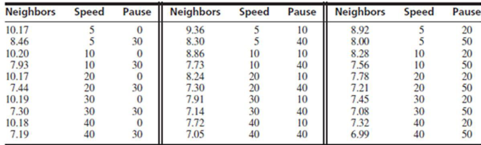
In a simulation of 30 mobile computer networks, the average speed, pause time, and number of neighbor were measured. A “neighbor” is a computer within the transmission
- a. Fit the model with Neighbors as the dependent variable, and independent variables Speed, Pause, Speed,·Pause, Speed2, and Pause2.
- b. Construct a reduced model by dropping any variables whose P-values are large, and test the plausibility of the model with an F test.
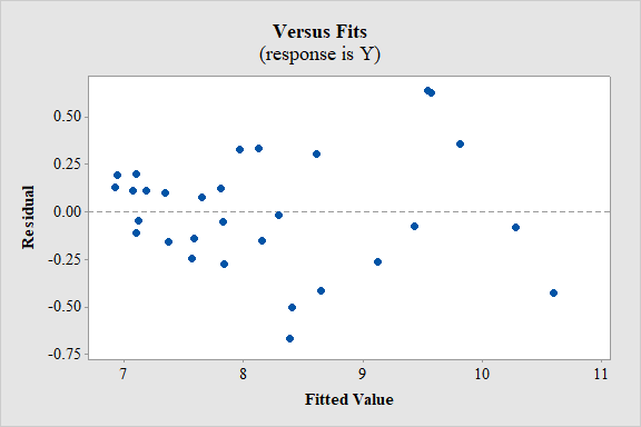
- c. Plot the residuals versus the fitted values for the reduced model. Are there any indications that the model is inappropriate? If so, what are they?
- d. Someone suggests that a model containing Pause and Pause2 as the only dependent variables is adequate. Do you agree? Why or why not?
- e. Using a best subsets software package, find the two models with the highest R2 value for each model size from one to five variables. Compute Cp and adjusted R2 for each model.
- f. Which model is selected by minimum Cp? By adjusted R2? Are they the same?
a.
Construct a multiple linear regression model with neighbor as the dependent variable, speed, pause,
Answer to Problem 5SE
A multiple linear regression model for the given data is:
Explanation of Solution
Calculation:
The data represents the values of the variables number of neighbors, average speed and pause time for a simulation of 30 mobile network computers.
Multiple linear regression model:
A multiple linear regression model is given as
Let
Regression:
Software procedure:
Step by step procedure to obtain regression using MINITAB software is given as,
- Choose Stat > Regression > General Regression.
- In Response, enter the numeric column containing the response data Y.
- In Model, enter the numeric column containing the predictor variables X1, X2, X1*X2, X1*X1 and X2*X2.
- Click OK.
Output obtained from MINITAB is given below:
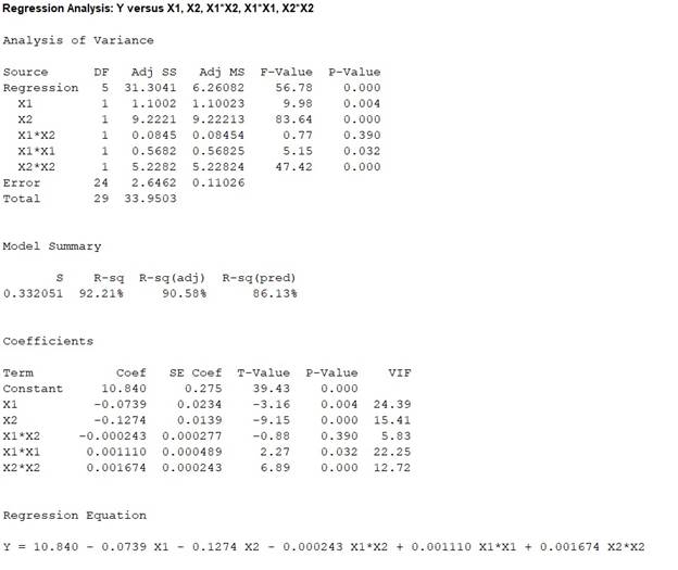
The ‘Coefficient’ column of the regression analysis MINITAB output gives the slopes corresponding to the respective variables stored in the column ‘Term’.
A careful inspection of the output shows that the fitted model is:
Hence, the multiple linear regression model for the given data is:
b.
Construct a reduced model by dropping the variables with large P- values.
Check whether the reduced model is plausible or not.
Answer to Problem 5SE
A multiple linear regression model for the given data is:
Yes, there is enough evidence to conclude that the reduced model is plausible.
Explanation of Solution
Calculation:
From part (a), it can be seen that the ‘P’ column of the regression analysis MINITAB output gives the slopes corresponding to the respective variables stored in the column ‘Term’.
By observing the P- values of the MINITAB output, it is clear that the largest P-value is 0.390 corresponding to the predictor variable
Now, the new regression has to be fitted after dropping the predictor variable
Regression:
Software procedure:
Step by step procedure to obtain regression using MINITAB software is given as,
- Choose Stat > Regression > General Regression.
- In Response, enter the numeric column containing the response data Y.
- In Model, enter the numeric column containing the predictor variables X1, X2, X1*X1 and X2*X2.
- Click OK.
Output obtained from MINITAB is given below:
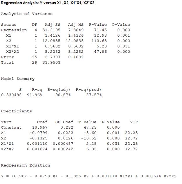
The ‘Coefficient’ column of the regression analysis MINITAB output gives the slopes corresponding to the respective variables stored in the column ‘Term’.
A careful inspection of the output shows that the fitted model is:
Hence, the multiple linear regression model for the given data is:
The full model is,
The reduced model is,
The test hypotheses are given below:
Null hypothesis:
That is, the dropped predictor of the full model is not significant to predict y.
Alternative hypothesis:
That is, the dropped predictor of the full model is significant to predict y.
Test statistic:
Where,
n represents the total number of observations.
p represents the number of predictors on the full model.
k represents the number of predictors on the reduced model.
From the obtained MINITAB outputs, the value of error sum of squares for full model is
The total number of observations is
Number of predictors on the full model is
Degrees of freedom of F-statistic for reduced model:
In a reduced multiple linear regression analysis, the F-statistic is
In the ratio, the numerator is obtained by dividing the quantity
Thus, the degrees of freedom for the F-statistic in a reduced multiple regression analysis are
Hence, the numerator degrees of freedom is
Test statistic under null hypothesis:
Under the null hypothesis, the test statistic is obtained as follows:
Thus, the test statistic is
Since, the level of significance is not specified. The prior level of significance
P-value:
Software procedure:
- Choose Graph > Probability Distribution Plot choose View Probability > OK.
- From Distribution, choose F, enter 1 in numerator df and 24 in denominator df.
- Click the Shaded Area tab.
- Choose X-Value and Right Tail for the region of the curve to shade.
- Enter the X-value as 0.76638.
- Click OK.
Output obtained from MINITAB is given below:
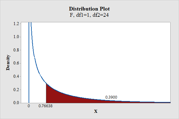
From the output, the P- value is 0.39.
Thus, the P- value is 0.39.
Decision criteria based on P-value approach:
If
If
Conclusion:
The P-value is 0.39 and
Here, P-value is greater than the
That is
By the rejection rule, fail to reject the null hypothesis.
Hence, there is sufficient evidence to conclude that the dropped predictor variable is not significant to predict the response variable y.
Thus, the reduced model is useful than the full model to predict the response variable y.
c.
Plot the residuals versus fitted line plot for the reduced model.
Check whether the model is appropriate.
Answer to Problem 5SE
Residual plot:
Yes, the model seems to be appropriate.
Explanation of Solution
Calculation:
Residual plot:
Software procedure:
Step by step procedure to obtain regression using MINITAB software is given as,
- Choose Stat > Regression > General Regression.
- In Response, enter the numeric column containing the response data Y.
- In Model, enter the numeric column containing the predictor variables X1, X2, X1*X1 and X2*X2.
- In Graphs, Under Residuals for plots, select Regular.
- Under Residual plots select box Residuals versus fits.
- Click OK.
Conditions for the appropriateness of regression model using the residual plot:
- The plot of the residuals vs. fitted values should fall roughly in a horizontal band contended and symmetric about x-axis. That is, the residuals of the data should not represent any bend.
- The plot of residuals should not contain any outliers.
- The residuals have to be scattered randomly around “0” with constant variability among for all the residuals. That is, the spread should be consistent.
Interpretation:
In residual plot there is high bend or pattern, which can violate the straight line condition and there is change in the spread of the residuals from one part to another part of the plot.
However, it is difficult to determine about the violation of the assumptions without the data.
Thus, the model seems to be appropriate.
d.
Check whether the model with only two dependent variables
Answer to Problem 5SE
No, the model with only two dependent variables
Explanation of Solution
Calculation:
Regression:
Software procedure:
Step by step procedure to obtain regression using MINITAB software is given as,
- Choose Stat > Regression > General Regression.
- In Response, enter the numeric column containing the response data Y.
- In Model, enter the numeric column containing the predictor variables X2 and X2*X2.
- Click OK.
Output obtained from MINITAB is given below:
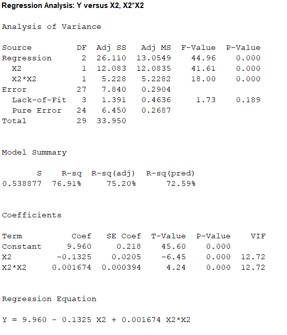
The ‘Coefficient’ column of the regression analysis MINITAB output gives the slopes corresponding to the respective variables stored in the column ‘Term’.
A careful inspection of the output shows that the fitted model is:
Hence, the multiple linear regression model for the given data is:
The full model is,
The reduced model is,
The test hypotheses are given below:
Null hypothesis:
That is, the dropped predictors of the full model are not significant to predict y.
Alternative hypothesis:
That is, at least one of the dropped predictors of the full model are significant to predict y.
Test statistic:
Where,
n represents the total number of observations.
p represents the number of predictors on the full model.
k represents the number of predictors on the reduced model.
From the obtained MINITAB outputs, the value of error sum of squares for full model is
The total number of observations is
Number of predictors on the full model is
Degrees of freedom of F-statistic for reduced model:
In a reduced multiple linear regression analysis, the F-statistic is
In the ratio, the numerator is obtained by dividing the quantity
Thus, the degrees of freedom for the F-statistic in a reduced multiple regression analysis are
Hence, the numerator degrees of freedom is
Test statistic under null hypothesis:
Under the null hypothesis, the test statistic is obtained as follows:
Thus, the test statistic is
Since, the level of significance is not specified. The prior level of significance
P-value:
Software procedure:
- Choose Graph > Probability Distribution Plot choose View Probability > OK.
- From Distribution, choose F, enter 3 in numerator df and 24 in denominator df.
- Click the Shaded Area tab.
- Choose X-Value and Right Tail for the region of the curve to shade.
- Enter the X-value as 15.702.
- Click OK.
Output obtained from MINITAB is given below:
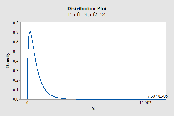
From the output, the P- value is
Thus, the P- value is
Decision criteria based on P-value approach:
If
If
Conclusion:
The P-value is
Here, P-value is less than the
That is
By the rejection rule, reject the null hypothesis.
Hence, there is sufficient evidence to conclude that at least one of the dropped predictors of the full model are significant to predict y.
Thus, the model with only two dependent variables
e.
Find the two models with the highest
Obtain the values of mallows
Answer to Problem 5SE
The two models with the highest
First model with
The values of M Mallows’
| Predictor variables | Mallows’ | Adjusted |
| 92.5 | 60.1 | |
| 97 | 58.6 | |
| 47.1 | 75.2 | |
| 53.3 | 73 | |
| 7.9 | 89.2 | |
| 15.5 | 86.4 | |
| 4.8 | 90.7 | |
| 9.2 | 89 | |
| 6 | 90.6 |
Explanation of Solution
Calculation:
Coefficient of multiple determination
The coefficient of multiple determination,
The subset with larger
Regression:
Software procedure:
Step by step procedure to obtain regression using MINITAB software is given as,
- Choose Stat > Regression > Regression> Best subsets.
- In Response, enter the numeric column containing the response data Y.
- In Model, enter the numeric column containing the predictor variables X1, X2, X1*X2, X1*X1 and X2*X2.
- Click OK.
Output obtained from MINITAB is given below:
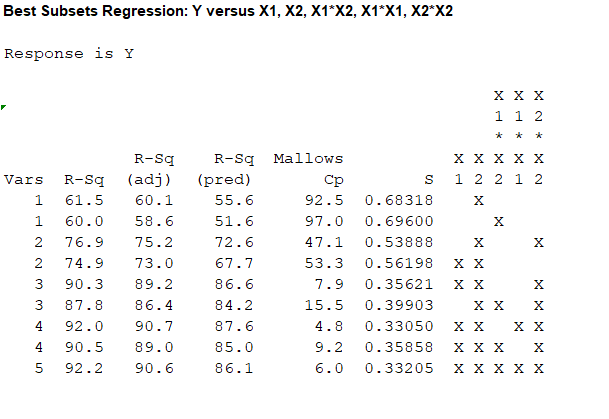
For the one predictor case, the highest value of
For the two predictor case, the highest value of
For the three predictor case, the highest value of
For the four predictor case, the highest value of
For the five predictor case, the value of
The value of
Thus, depending upon the factors affecting the analysis it would be most preferable to use the regression equation corresponding to the predictors
The second highest value of
That is, 90.6 and 90.3 are not much distinct.
Therefore, the model with
Thus, the two best models are:
First model with
From the accompanying MINITAB output, the values of Mallows’
| Predictor variables | Mallows’ | Adjusted |
| 92.5 | 60.1 | |
| 97 | 58.6 | |
| 47.1 | 75.2 | |
| 53.3 | 73 | |
| 7.9 | 89.2 | |
| 15.5 | 86.4 | |
| 4.8 | 90.7 | |
| 9.2 | 89 | |
| 6 | 90.6 |
f.
Select the variables for the model, using the Mallows’
Check whether both the models are same.
Answer to Problem 5SE
The variables for the model using the Mallows’
The variables for the model using the adjusted-
Yes, both the models are same.
Explanation of Solution
Mallows’
An important utility of the Mallows’
Mallows’
The predictor with the lowest value of
From part (e), the values of Mallows’
| Predictor variables | Mallows’ | Adjusted |
| 92.5 | 60.1 | |
| 97 | 58.6 | |
| 47.1 | 75.2 | |
| 53.3 | 73 | |
| 7.9 | 89.2 | |
| 15.5 | 86.4 | |
| 4.8 | 90.7 | |
| 9.2 | 89 | |
| 6 | 90.6 |
For the one predictor case, the lowest value of
For the two predictor case, the lowest value of
For the three predictor case, the lowest value of
For the four predictor case, the lowest value of
For the five predictor case, the value of
The value of
Thus, depending upon the factors affecting the analysis it would be most preferable to use the regression equation corresponding to the predictors
Hence, the variables for the model using the Mallows’
Adjusted
An important utility of the adjusted coefficient of multiple determination or
The adjusted coefficient of multiple determination,
For the one predictor case, the highest value of
For the two predictor case, the highest value of
For the three predictor case, the highest value of
For the four predictor case, the highest value of
For the five predictor case, the value of
The value of adjusted
Thus, provided other factors do not affect the analysis it could be most preferable to use the regression equation corresponding to the predictors,
Hence, the variables for the model using the adjusted-
Both Mallows’
Want to see more full solutions like this?
Chapter 8 Solutions
EBK STATISTICS FOR ENGINEERS AND SCIENT
Additional Math Textbook Solutions
Math in Our World
Elementary Statistics ( 3rd International Edition ) Isbn:9781260092561
APPLIED STAT.IN BUS.+ECONOMICS
Introductory Statistics
Elementary Statistics: Picturing the World (7th Edition)
Mathematics for the Trades: A Guided Approach (11th Edition) (What's New in Trade Math)


- PS 9 Two films are shown on screen A and screen B at a cinema each evening. The numbers of people viewing the films on 12 consecutive evenings are shown in the back-to-back stem-and-leaf diagram. Screen A (12) Screen B (12) 8 037 34 7 6 4 0 534 74 1645678 92 71689 Key: 116|4 represents 61 viewers for A and 64 viewers for B A second stem-and-leaf diagram (with rows of the same width as the previous diagram) is drawn showing the total number of people viewing films at the cinema on each of these 12 evenings. Find the least and greatest possible number of rows that this second diagram could have. TIP On the evening when 30 people viewed films on screen A, there could have been as few as 37 or as many as 79 people viewing films on screen B.arrow_forwardQ.2.4 There are twelve (12) teams participating in a pub quiz. What is the probability of correctly predicting the top three teams at the end of the competition, in the correct order? Give your final answer as a fraction in its simplest form.arrow_forwardThe table below indicates the number of years of experience of a sample of employees who work on a particular production line and the corresponding number of units of a good that each employee produced last month. Years of Experience (x) Number of Goods (y) 11 63 5 57 1 48 4 54 5 45 3 51 Q.1.1 By completing the table below and then applying the relevant formulae, determine the line of best fit for this bivariate data set. Do NOT change the units for the variables. X y X2 xy Ex= Ey= EX2 EXY= Q.1.2 Estimate the number of units of the good that would have been produced last month by an employee with 8 years of experience. Q.1.3 Using your calculator, determine the coefficient of correlation for the data set. Interpret your answer. Q.1.4 Compute the coefficient of determination for the data set. Interpret your answer.arrow_forward
- Can you answer this question for mearrow_forwardTechniques QUAT6221 2025 PT B... TM Tabudi Maphoru Activities Assessments Class Progress lIE Library • Help v The table below shows the prices (R) and quantities (kg) of rice, meat and potatoes items bought during 2013 and 2014: 2013 2014 P1Qo PoQo Q1Po P1Q1 Price Ро Quantity Qo Price P1 Quantity Q1 Rice 7 80 6 70 480 560 490 420 Meat 30 50 35 60 1 750 1 500 1 800 2 100 Potatoes 3 100 3 100 300 300 300 300 TOTAL 40 230 44 230 2 530 2 360 2 590 2 820 Instructions: 1 Corall dawn to tha bottom of thir ceraan urina se se tha haca nariad in archerca antarand cubmit Q Search ENG US 口X 2025/05arrow_forwardThe table below indicates the number of years of experience of a sample of employees who work on a particular production line and the corresponding number of units of a good that each employee produced last month. Years of Experience (x) Number of Goods (y) 11 63 5 57 1 48 4 54 45 3 51 Q.1.1 By completing the table below and then applying the relevant formulae, determine the line of best fit for this bivariate data set. Do NOT change the units for the variables. X y X2 xy Ex= Ey= EX2 EXY= Q.1.2 Estimate the number of units of the good that would have been produced last month by an employee with 8 years of experience. Q.1.3 Using your calculator, determine the coefficient of correlation for the data set. Interpret your answer. Q.1.4 Compute the coefficient of determination for the data set. Interpret your answer.arrow_forward
- Q.3.2 A sample of consumers was asked to name their favourite fruit. The results regarding the popularity of the different fruits are given in the following table. Type of Fruit Number of Consumers Banana 25 Apple 20 Orange 5 TOTAL 50 Draw a bar chart to graphically illustrate the results given in the table.arrow_forwardQ.2.3 The probability that a randomly selected employee of Company Z is female is 0.75. The probability that an employee of the same company works in the Production department, given that the employee is female, is 0.25. What is the probability that a randomly selected employee of the company will be female and will work in the Production department? Q.2.4 There are twelve (12) teams participating in a pub quiz. What is the probability of correctly predicting the top three teams at the end of the competition, in the correct order? Give your final answer as a fraction in its simplest form.arrow_forwardQ.2.1 A bag contains 13 red and 9 green marbles. You are asked to select two (2) marbles from the bag. The first marble selected will not be placed back into the bag. Q.2.1.1 Construct a probability tree to indicate the various possible outcomes and their probabilities (as fractions). Q.2.1.2 What is the probability that the two selected marbles will be the same colour? Q.2.2 The following contingency table gives the results of a sample survey of South African male and female respondents with regard to their preferred brand of sports watch: PREFERRED BRAND OF SPORTS WATCH Samsung Apple Garmin TOTAL No. of Females 30 100 40 170 No. of Males 75 125 80 280 TOTAL 105 225 120 450 Q.2.2.1 What is the probability of randomly selecting a respondent from the sample who prefers Garmin? Q.2.2.2 What is the probability of randomly selecting a respondent from the sample who is not female? Q.2.2.3 What is the probability of randomly…arrow_forward
- Test the claim that a student's pulse rate is different when taking a quiz than attending a regular class. The mean pulse rate difference is 2.7 with 10 students. Use a significance level of 0.005. Pulse rate difference(Quiz - Lecture) 2 -1 5 -8 1 20 15 -4 9 -12arrow_forwardThe following ordered data list shows the data speeds for cell phones used by a telephone company at an airport: A. Calculate the Measures of Central Tendency from the ungrouped data list. B. Group the data in an appropriate frequency table. C. Calculate the Measures of Central Tendency using the table in point B. D. Are there differences in the measurements obtained in A and C? Why (give at least one justified reason)? I leave the answers to A and B to resolve the remaining two. 0.8 1.4 1.8 1.9 3.2 3.6 4.5 4.5 4.6 6.2 6.5 7.7 7.9 9.9 10.2 10.3 10.9 11.1 11.1 11.6 11.8 12.0 13.1 13.5 13.7 14.1 14.2 14.7 15.0 15.1 15.5 15.8 16.0 17.5 18.2 20.2 21.1 21.5 22.2 22.4 23.1 24.5 25.7 28.5 34.6 38.5 43.0 55.6 71.3 77.8 A. Measures of Central Tendency We are to calculate: Mean, Median, Mode The data (already ordered) is: 0.8, 1.4, 1.8, 1.9, 3.2, 3.6, 4.5, 4.5, 4.6, 6.2, 6.5, 7.7, 7.9, 9.9, 10.2, 10.3, 10.9, 11.1, 11.1, 11.6, 11.8, 12.0, 13.1, 13.5, 13.7, 14.1, 14.2, 14.7, 15.0, 15.1, 15.5,…arrow_forwardPEER REPLY 1: Choose a classmate's Main Post. 1. Indicate a range of values for the independent variable (x) that is reasonable based on the data provided. 2. Explain what the predicted range of dependent values should be based on the range of independent values.arrow_forward
 Functions and Change: A Modeling Approach to Coll...AlgebraISBN:9781337111348Author:Bruce Crauder, Benny Evans, Alan NoellPublisher:Cengage Learning
 Holt Mcdougal Larson Pre-algebra: Student Edition...AlgebraISBN:9780547587776Author:HOLT MCDOUGALPublisher:HOLT MCDOUGAL
 Big Ideas Math A Bridge To Success Algebra 1: Stu...AlgebraISBN:9781680331141Author:HOUGHTON MIFFLIN HARCOURTPublisher:Houghton Mifflin Harcourt