
Videos
The article “Effect of Environmental Factors on Steel Plate Corrosion Under Marine Immersion Conditions” (C. Soares, Y. Garbatov, and A. Zayed, Corrosion Engineering, Science and Technology, 2011:524–541) describes an experiment in which nine steel specimens were submerged in seawater at various temperatures, and the corrosion rates were measured. The results are presented in the following table (obtained by digitizing a graph).
| Temperature (°C) | Corrosion (mm/yr) |
| 26.6 | 1.58 |
| 26.0 | 1.45 |
| 27.4 | 1.13 |
| 21.7 | 0.96 |
| 14.9 | 0.99 |
| 11.3 | 1.05 |
| 15.0 | 0.82 |
| 8.7 | 0.68 |
| 8.2 | 0.56 |
- a. Construct a
scatterplot of corrosion (y) versus temperature (x). Verify that a linear model is appropriate. - b. Compute the least-squares line for predicting corrosion from temperature.
- c. Two steel specimens whose temperatures differ by 10°C are submerged in seawater. By how much would you predict their corrosion rates to differ?
- d. Predict the corrosion rate for steel submerged in seawater at a temperature of 20°C.
- e. Compute the fitted values.
- f. Compute the residuals. Which point has the residual with the largest magnitude?
- g. Compute the
correlation between temperature and corrosion rate. - h. Compute the regression sum of squares, the error sum of squares, and the total sum of squares.
- i. Divide the regression sum of squares by the total sum of squares. What is the relationship between this quantity and the
correlation coefficient ?
a.
Construct a scatterplot of corrosion (y) versus temperature (x) and also check whether the linear model is appropriate or not.
Answer to Problem 10E
The linear model is appropriate.
Explanation of Solution
Calculation:
The given information is that the data shows the temperature (°C) and corrosion (mm/yr) for 9 steel specimens.
Software Procedure:
Step-by-step procedure to obtain the scatterplot using the MINITAB software:
- Choose Graph > Scatter plot.
- Choose Simple, and then click OK.
- Under Y variables, select Corrosion.
- Under X variables, select Temperature.
- Click OK.
Output using the MINITAB software is given below:
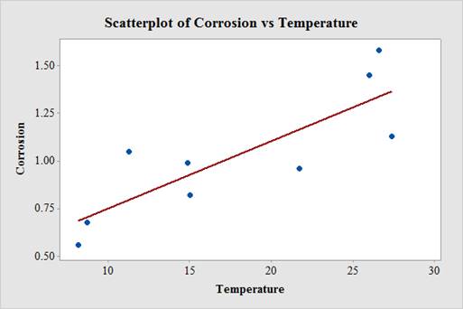
From the plot, it can be observed that the relationship between temperature and corrosion is linear. Therefore, the linear model is appropriate.
b.
Find the least-squares line for predicting corrosion from temperature.
Answer to Problem 10E
The least-squares line for predicting corrosion from temperature is
Explanation of Solution
Calculation:
Software Procedure:
Step-by-step procedure to obtain the least-squares line using the MINITAB software is given below:
- Choose Stat > Regression > Regression > Fit Regression Model.
- In Responses, enter “Corrosion”.
- In Continuous predictors, enter “Temperature”.
- Check Results.
- In Display of results, choose Simple tables.
- Click OK.
Output using the MINITAB software is given below:
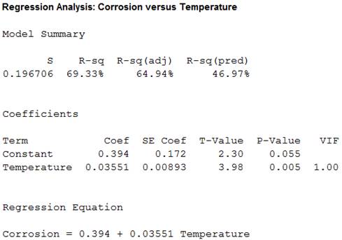
From the MINITAB output, the least-squares line for predicting corrosion from temperature is
c.
By how much would predict corrosion rates of two steel specimens to differ whose temperatures differ by 10ºC.
Explanation of Solution
Calculation:
From the least square line, the slope
The change in the predicted corrosion rates when two steel specimens whose temperatures differ by 10ºC is
Thus, the predicted corrosion rate is 0.3351 mm/yr.
d.
Predict the corrosion rate for steel submerged in seawater at a temperature of 20ºC.
Answer to Problem 10E
The predicted corrosion rate for steel submerged in seawater at a temperature of 20ºC is 1.10414 mm/yr.
Explanation of Solution
Calculation:
Predicted value:
Software Procedure:
Step-by-step procedure to obtain the predicted value using the MINITAB software:
- Stat > Regression > Regression > Predict.
- In Responses, enter “Corrosion”.
- Choose Enter individual values.
- In Temperature, enter 20.
- Click OK.
Output using the MINITAB software is given below:
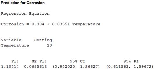
From the MINITAB output, the predicted corrosion rate for steel submerged in seawater at a temperature of 20ºC is 1.10414 mm/yr.
e.
Find the fitted values.
Answer to Problem 10E
The fitted values are, 1.33850, 1.31720, 1.36691, 1.16451, 0.92305, 0.79521, 0.92660, 0.70289 and 0.68513.
Explanation of Solution
Calculation:
Fitted value:
Software Procedure:
Step-by-step procedure to obtain the fitted value using the MINITAB software is given below:
- Choose Stat > Regression > Regression > Fit Regression Model.
- In Responses, enter “Corrosion”.
- In Continuous predictors, enter “Temperature”.
- Check Results.
- In Display of results, choose Simple tables.
- In Storage, select fits.
- Click OK.
Data display:
- Choose Data > Display data.
- In Columns, constants, and matrices to display, select FITS 1.
Output using the MINITAB software is given below:

The fitted values are, 1.33850, 1.31720, 1.36691, 1.16451, 0.92305, 0.79521, 0.92660, 0.70289 and 0.68513.
f.
Find the residuals and identify the point whose residual has the largest magnitude.
Answer to Problem 10E
The residual points are 0.241497, 0.132802, –0.236911, –0.204508, 0.066954,0.254787, –0.106597, –0.022889 and –0.125135.
The point whose residual has the largest magnitude is (11.3, 1.05).
Explanation of Solution
Calculation:
Residuals:
Software Procedure:
Step-by-step procedure to obtain the fitted value using the MINITAB software is given below:
- Choose Stat > Regression > Regression > Fit Regression Model.
- In Responses, enter “Corrosion”.
- In Continuous predictors, enter “Temperature”.
- Check Results.
- In Display of results, choose Simple tables.
- In Storage, select residuals.
- Click OK.
Data display:
- Choose Data > Display data.
- In Columns, constants, and matrices to display, select RESI 1.
Output using the MINITAB software is given below:
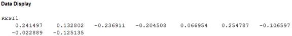
The residual points are 0.241497, 0.132802, –0.236911, –0.204508, 0.066954, 0.254787, –0.106597, –0.022889 and –0.125135.
Therefore, the point whose residual has the largest magnitude is (11.3, 1.05) because this point has the largest residual.
g.
Find the correlation between temperature and corrosion rate.
Answer to Problem 10E
The correlation between temperature and corrosion rate is 0.833.
Explanation of Solution
Calculation:
Correlation:
Software Procedure:
Step-by-step procedure to obtain the correlation using the MINITAB software:
- Select Stat > Basic Statistics > Correlation.
- In Variables, select Temperature and corrosion rate.
- Click OK.
Output using the MINITAB software is given below:
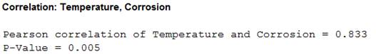
Thus, the correlation between temperature and corrosion rate is 0.833.
h.
Find the regression sum of squares, the error sum of squares, and the total sum of squares.
Answer to Problem 10E
The regression sum of squares is 0.6122, the error sum of squares is 0.2709 and the total sum of squares is 0.8830.
Explanation of Solution
Calculation:
Step-by-step procedure to obtain the regression sum of squares, the error sum of squares, and the total sum of squares using the MINITAB software is given below:
- Choose Stat > Regression > Regression > Fit Regression Model.
- In Responses, enter “Corrosion”.
- In Continuous predictors, enter “Temperature”.
- Check Results.
- In Display of results, choose Simple tables.
- Click OK.
Output using the MINITAB software is given below:
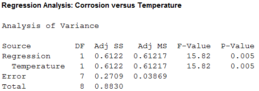
From the output, the regression sum of squares is 0.6122, the error sum of squares is 0.2709 and the total sum of squares is 0.8830.
i.
Identify the relationship between the quantity
Answer to Problem 10E
The quantity
Explanation of Solution
Calculation:
The regression sum of squares divided by the total sum of squares is
This value almost closer to the
The relationship between the quantity
Thus, the quantity
Want to see more full solutions like this?
Chapter 7 Solutions
Statistics for Engineers and Scientists
Additional Math Textbook Solutions
Pathways To Math Literacy (looseleaf)
Precalculus: Mathematics for Calculus (Standalone Book)
College Algebra Essentials (5th Edition)
Elementary Statistics ( 3rd International Edition ) Isbn:9781260092561
College Algebra (7th Edition)
APPLIED STAT.IN BUS.+ECONOMICS


- According to an economist from a financial company, the average expenditures on "furniture and household appliances" have been lower for households in the Montreal area than those in the Quebec region. A random sample of 14 households from the Montreal region and 16 households from the Quebec region was taken, providing the following data regarding expenditures in this economic sector. It is assumed that the data from each population are distributed normally. We are interested in knowing if the variances of the populations are equal. a) Perform the appropriate hypothesis test on two variances at a significance level of 1%. Include the following information: i. Hypothesis / Identification of populations ii. Critical F-value(s) iii. Decision rule iv. F-ratio value v. Decision and conclusion b) Based on the results obtained in a), is the hypothesis of equal variances for this socio-economic characteristic measured in these two populations upheld? c) Based on the results obtained in a),…arrow_forwardA major company in the Montreal area, offering a range of engineering services from project preparation to construction execution, and industrial project management, wants to ensure that the individuals who are responsible for project cost estimation and bid preparation demonstrate a certain uniformity in their estimates. The head of civil engineering and municipal services decided to structure an experimental plan to detect if there could be significant differences in project evaluation. Seven projects were selected, each of which had to be evaluated by each of the two estimators, with the order of the projects submitted being random. The obtained estimates are presented in the table below. a) Complete the table above by calculating: i. The differences (A-B) ii. The sum of the differences iii. The mean of the differences iv. The standard deviation of the differences b) What is the value of the t-statistic? c) What is the critical t-value for this test at a significance level of 1%?…arrow_forwardCompute the relative risk of falling for the two groups (did not stop walking vs. did stop). State/interpret your result verbally.arrow_forward
- Microsoft Excel include formulasarrow_forwardQuestion 1 The data shown in Table 1 are and R values for 24 samples of size n = 5 taken from a process producing bearings. The measurements are made on the inside diameter of the bearing, with only the last three decimals recorded (i.e., 34.5 should be 0.50345). Table 1: Bearing Diameter Data Sample Number I R Sample Number I R 1 34.5 3 13 35.4 8 2 34.2 4 14 34.0 6 3 31.6 4 15 37.1 5 4 31.5 4 16 34.9 7 5 35.0 5 17 33.5 4 6 34.1 6 18 31.7 3 7 32.6 4 19 34.0 8 8 33.8 3 20 35.1 9 34.8 7 21 33.7 2 10 33.6 8 22 32.8 1 11 31.9 3 23 33.5 3 12 38.6 9 24 34.2 2 (a) Set up and R charts on this process. Does the process seem to be in statistical control? If necessary, revise the trial control limits. [15 pts] (b) If specifications on this diameter are 0.5030±0.0010, find the percentage of nonconforming bearings pro- duced by this process. Assume that diameter is normally distributed. [10 pts] 1arrow_forward4. (5 pts) Conduct a chi-square contingency test (test of independence) to assess whether there is an association between the behavior of the elderly person (did not stop to talk, did stop to talk) and their likelihood of falling. Below, please state your null and alternative hypotheses, calculate your expected values and write them in the table, compute the test statistic, test the null by comparing your test statistic to the critical value in Table A (p. 713-714) of your textbook and/or estimating the P-value, and provide your conclusions in written form. Make sure to show your work. Did not stop walking to talk Stopped walking to talk Suffered a fall 12 11 Totals 23 Did not suffer a fall | 2 Totals 35 37 14 46 60 Tarrow_forward
- Question 2 Parts manufactured by an injection molding process are subjected to a compressive strength test. Twenty samples of five parts each are collected, and the compressive strengths (in psi) are shown in Table 2. Table 2: Strength Data for Question 2 Sample Number x1 x2 23 x4 x5 R 1 83.0 2 88.6 78.3 78.8 3 85.7 75.8 84.3 81.2 78.7 75.7 77.0 71.0 84.2 81.0 79.1 7.3 80.2 17.6 75.2 80.4 10.4 4 80.8 74.4 82.5 74.1 75.7 77.5 8.4 5 83.4 78.4 82.6 78.2 78.9 80.3 5.2 File Preview 6 75.3 79.9 87.3 89.7 81.8 82.8 14.5 7 74.5 78.0 80.8 73.4 79.7 77.3 7.4 8 79.2 84.4 81.5 86.0 74.5 81.1 11.4 9 80.5 86.2 76.2 64.1 80.2 81.4 9.9 10 75.7 75.2 71.1 82.1 74.3 75.7 10.9 11 80.0 81.5 78.4 73.8 78.1 78.4 7.7 12 80.6 81.8 79.3 73.8 81.7 79.4 8.0 13 82.7 81.3 79.1 82.0 79.5 80.9 3.6 14 79.2 74.9 78.6 77.7 75.3 77.1 4.3 15 85.5 82.1 82.8 73.4 71.7 79.1 13.8 16 78.8 79.6 80.2 79.1 80.8 79.7 2.0 17 82.1 78.2 18 84.5 76.9 75.5 83.5 81.2 19 79.0 77.8 20 84.5 73.1 78.2 82.1 79.2 81.1 7.6 81.2 84.4 81.6 80.8…arrow_forwardName: Lab Time: Quiz 7 & 8 (Take Home) - due Wednesday, Feb. 26 Contingency Analysis (Ch. 9) In lab 5, part 3, you will create a mosaic plot and conducted a chi-square contingency test to evaluate whether elderly patients who did not stop walking to talk (vs. those who did stop) were more likely to suffer a fall in the next six months. I have tabulated the data below. Answer the questions below. Please show your calculations on this or a separate sheet. Did not stop walking to talk Stopped walking to talk Totals Suffered a fall Did not suffer a fall Totals 12 11 23 2 35 37 14 14 46 60 Quiz 7: 1. (2 pts) Compute the odds of falling for each group. Compute the odds ratio for those who did not stop walking vs. those who did stop walking. Interpret your result verbally.arrow_forwardSolve please and thank you!arrow_forward
- 7. In a 2011 article, M. Radelet and G. Pierce reported a logistic prediction equation for the death penalty verdicts in North Carolina. Let Y denote whether a subject convicted of murder received the death penalty (1=yes), for the defendant's race h (h1, black; h = 2, white), victim's race i (i = 1, black; i = 2, white), and number of additional factors j (j = 0, 1, 2). For the model logit[P(Y = 1)] = a + ß₁₂ + By + B²², they reported = -5.26, D â BD = 0, BD = 0.17, BY = 0, BY = 0.91, B = 0, B = 2.02, B = 3.98. (a) Estimate the probability of receiving the death penalty for the group most likely to receive it. [4 pts] (b) If, instead, parameters used constraints 3D = BY = 35 = 0, report the esti- mates. [3 pts] h (c) If, instead, parameters used constraints Σ₁ = Σ₁ BY = Σ; B = 0, report the estimates. [3 pts] Hint the probabilities, odds and odds ratios do not change with constraints.arrow_forwardSolve please and thank you!arrow_forwardSolve please and thank you!arrow_forward
 MATLAB: An Introduction with ApplicationsStatisticsISBN:9781119256830Author:Amos GilatPublisher:John Wiley & Sons Inc
 Probability and Statistics for Engineering and th...StatisticsISBN:9781305251809Author:Jay L. DevorePublisher:Cengage Learning
 Statistics for The Behavioral Sciences (MindTap C...StatisticsISBN:9781305504912Author:Frederick J Gravetter, Larry B. WallnauPublisher:Cengage Learning
 Elementary Statistics: Picturing the World (7th E...StatisticsISBN:9780134683416Author:Ron Larson, Betsy FarberPublisher:PEARSON
 The Basic Practice of StatisticsStatisticsISBN:9781319042578Author:David S. Moore, William I. Notz, Michael A. FlignerPublisher:W. H. Freeman
 Introduction to the Practice of StatisticsStatisticsISBN:9781319013387Author:David S. Moore, George P. McCabe, Bruce A. CraigPublisher:W. H. Freeman