Videos
(a)
To graph: The histogram.
(a)
Explanation of Solution
Calculation:
To draw the histogram, follow the below mentioned steps in Minitab:
Step 1: Enter the data in Minitab and enter variable name as “Diameter.”
Step 2: Go to “Graph” and point on “Histogram.” Click on “Simple” and then press OK.
Step 3: In dialog box that appears, select “Diameter” under the field marked as “Graph variable,” and then click on OK.
The histogram obtained is as follows:
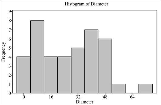
Interpretation: The histogram does not seem to represent a bell-shaped curve.
To graph: The box plot.
Explanation of Solution
Graph: To draw the box plot, follow the below mentioned steps in Minitab:
Step 1: Enter the data in Minitab and enter variable name as “Diameter.”
Step 2: Go to
Step 3: In dialog box that appears, select “Diameter” under the field marked as “Graph variable,” and then click on OK.
The required box plot is as follows:
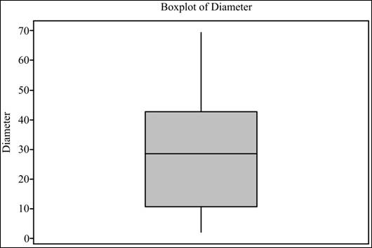
Interpretation: From the box plot, the data does not appear to be symmetrical.
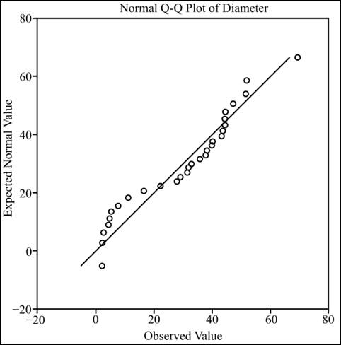
To graph: The normal quantile plot.
Explanation of Solution
Given: The data for the diameters of 40 randomly sampled trees is provided.
Calculation: To draw the normal quantile plot, follow the below mentioned steps in SPSS.
Step 1: Enter the data of diameter in SPSS and enter the variable name “Diameter.”
Step 2: Go to
Step 3: Select “Diameter” under the field marked as “Variables.” Finally, click on “Ok.”
The normal quantile plots are as follows:
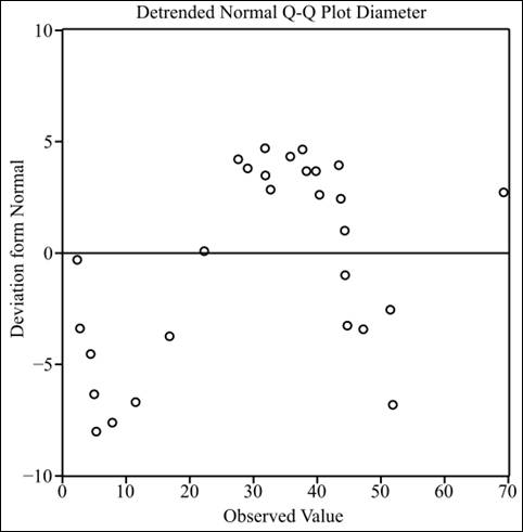
To explain: The distribution.
Answer to Problem 33E
Solution: The distribution is not normal as it has two peaks, and the normal quantile plot shows that the distribution is deviated from the
Explanation of Solution
The histogram of the distribution shows that it has two peaks. In the box plot, the upper tail is longer than the lower tail, which indicates its deviation from normality, and the normal quantile plots also show that the data is deviated from the normal distribution as most of the values are away from the normal position.
(b)
Whether t procedures can be used to calculate 95% confidence interval.
(b)
Answer to Problem 33E
Solution: The t procedures can be used as the sample is large enough to eliminate the effect of non-normal distribution.
Explanation of Solution
As the data is large enough as compared to the population, it will eliminate the effect of non-normality. So, the t procedures can be used.
(c)
Section 1:
To find: The margin of error.
(c)
Section 1:
Answer to Problem 33E
Solution: The margin of error is 5.68.
Explanation of Solution
Calculation:
To calculate the margin of error, first, standard deviation and
Step 1: Enter the data in Minitab and enter variable name as “Diameter.”
Step 2: Go to
Step 3: In dialog box that appears, select “Diameter” under the field marked as “Variables,” and then click on “Statistics.”
Step 4: In dialog box that appears, select “None” and then “Mean” and “Standard deviation.” Finally, click on “Ok” on both dialog boxes.
From Minitab result, the standard deviation is 17.71 and the mean is 27.29.
The formula for margin of error is as follows:
where
Section 2:
To find: The 95% confidence interval for mean diameter.
Section 2:
Answer to Problem 33E
Solution: The 95% confidence interval is
Explanation of Solution
Calculation:
The confidence interval is an interval for which there are 95% chances that it contains the population parameter (population mean).
To calculate confidence interval, follow the below mentioned steps in Minitab:
Step 1: Enter the provided data into Minitab and enter variable name as “Diameter.”
Step 2: Go to
Step 3: In the dialog box that appears, select “Diameter” under the field marked as “sample in columns.” Click on “option.”
Step 4: In the dialog box that appears, enter “95.0” in confidence level and select “not equal” in “Alternative hypothesis.”
From Minitab results, 95% confidence interval is
Interpretation: The 95% confidence interval is
(d)
Whether the result found in parts (a), (b), and (c) would apply to the trees in the same area.
(d)
Answer to Problem 33E
Solution: The result would not apply to the trees in the same area because the sample size was small and the data was also not normal.
Explanation of Solution
The sample size must be large to conclude about the population but here the sample size was not large enough to conclude about the trees in the same area. Therefore, the result would not be applied to other trees in the same area.
Want to see more full solutions like this?
Chapter 7 Solutions
Introduction to the Practice of Statistics


- A school counselor is conducting a research study to examine whether there is a relationship between the number of times teenagers report vaping per week and their academic performance, measured by GPA. The counselor collects data from a sample of high school students. Write the null and alternative hypotheses for this study. Clearly state your hypotheses in terms of the correlation between vaping frequency and academic performance. EditViewInsertFormatToolsTable 12pt Paragrapharrow_forwardA smallish urn contains 25 small plastic bunnies – 7 of which are pink and 18 of which are white. 10 bunnies are drawn from the urn at random with replacement, and X is the number of pink bunnies that are drawn. (a) P(X = 5) ≈ (b) P(X<6) ≈ The Whoville small urn contains 100 marbles – 60 blue and 40 orange. The Grinch sneaks in one night and grabs a simple random sample (without replacement) of 15 marbles. (a) The probability that the Grinch gets exactly 6 blue marbles is [ Select ] ["≈ 0.054", "≈ 0.043", "≈ 0.061"] . (b) The probability that the Grinch gets at least 7 blue marbles is [ Select ] ["≈ 0.922", "≈ 0.905", "≈ 0.893"] . (c) The probability that the Grinch gets between 8 and 12 blue marbles (inclusive) is [ Select ] ["≈ 0.801", "≈ 0.760", "≈ 0.786"] . The Whoville small urn contains 100 marbles – 60 blue and 40 orange. The Grinch sneaks in one night and grabs a simple random sample (without replacement) of 15 marbles. (a)…arrow_forwardSuppose an experiment was conducted to compare the mileage(km) per litre obtained by competing brands of petrol I,II,III. Three new Mazda, three new Toyota and three new Nissan cars were available for experimentation. During the experiment the cars would operate under same conditions in order to eliminate the effect of external variables on the distance travelled per litre on the assigned brand of petrol. The data is given as below: Brands of Petrol Mazda Toyota Nissan I 10.6 12.0 11.0 II 9.0 15.0 12.0 III 12.0 17.4 13.0 (a) Test at the 5% level of significance whether there are signi cant differences among the brands of fuels and also among the cars. [10] (b) Compute the standard error for comparing any two fuel brands means. Hence compare, at the 5% level of significance, each of fuel brands II, and III with the standard fuel brand I. [10] �arrow_forward
- Analyze the residuals of a linear regression model and select the best response. yes, the residual plot does not show a curve no, the residual plot shows a curve yes, the residual plot shows a curve no, the residual plot does not show a curve I answered, "No, the residual plot shows a curve." (and this was incorrect). I am not sure why I keep getting these wrong when the answer seems obvious. Please help me understand what the yes and no references in the answer.arrow_forwarda. Find the value of A.b. Find pX(x) and py(y).c. Find pX|y(x|y) and py|X(y|x)d. Are x and y independent? Why or why not?arrow_forwardAnalyze the residuals of a linear regression model and select the best response.Criteria is simple evaluation of possible indications of an exponential model vs. linear model) no, the residual plot does not show a curve yes, the residual plot does not show a curve yes, the residual plot shows a curve no, the residual plot shows a curve I selected: yes, the residual plot shows a curve and it is INCORRECT. Can u help me understand why?arrow_forward
- You have been hired as an intern to run analyses on the data and report the results back to Sarah; the five questions that Sarah needs you to address are given below. please do it step by step on excel Does there appear to be a positive or negative relationship between price and screen size? Use a scatter plot to examine the relationship. Determine and interpret the correlation coefficient between the two variables. In your interpretation, discuss the direction of the relationship (positive, negative, or zero relationship). Also discuss the strength of the relationship. Estimate the relationship between screen size and price using a simple linear regression model and interpret the estimated coefficients. (In your interpretation, tell the dollar amount by which price will change for each unit of increase in screen size). Include the manufacturer dummy variable (Samsung=1, 0 otherwise) and estimate the relationship between screen size, price and manufacturer dummy as a multiple…arrow_forwardHere is data with as the response variable. x y54.4 19.124.9 99.334.5 9.476.6 0.359.4 4.554.4 0.139.2 56.354 15.773.8 9-156.1 319.2Make a scatter plot of this data. Which point is an outlier? Enter as an ordered pair, e.g., (x,y). (x,y)= Find the regression equation for the data set without the outlier. Enter the equation of the form mx+b rounded to three decimal places. y_wo= Find the regression equation for the data set with the outlier. Enter the equation of the form mx+b rounded to three decimal places. y_w=arrow_forwardYou have been hired as an intern to run analyses on the data and report the results back to Sarah; the five questions that Sarah needs you to address are given below. please do it step by step Does there appear to be a positive or negative relationship between price and screen size? Use a scatter plot to examine the relationship. Determine and interpret the correlation coefficient between the two variables. In your interpretation, discuss the direction of the relationship (positive, negative, or zero relationship). Also discuss the strength of the relationship. Estimate the relationship between screen size and price using a simple linear regression model and interpret the estimated coefficients. (In your interpretation, tell the dollar amount by which price will change for each unit of increase in screen size). Include the manufacturer dummy variable (Samsung=1, 0 otherwise) and estimate the relationship between screen size, price and manufacturer dummy as a multiple linear…arrow_forward
 MATLAB: An Introduction with ApplicationsStatisticsISBN:9781119256830Author:Amos GilatPublisher:John Wiley & Sons Inc
 Probability and Statistics for Engineering and th...StatisticsISBN:9781305251809Author:Jay L. DevorePublisher:Cengage Learning
 Statistics for The Behavioral Sciences (MindTap C...StatisticsISBN:9781305504912Author:Frederick J Gravetter, Larry B. WallnauPublisher:Cengage Learning
 Elementary Statistics: Picturing the World (7th E...StatisticsISBN:9780134683416Author:Ron Larson, Betsy FarberPublisher:PEARSON
 The Basic Practice of StatisticsStatisticsISBN:9781319042578Author:David S. Moore, William I. Notz, Michael A. FlignerPublisher:W. H. Freeman
 Introduction to the Practice of StatisticsStatisticsISBN:9781319013387Author:David S. Moore, George P. McCabe, Bruce A. CraigPublisher:W. H. Freeman