
Concept explainers
Videos
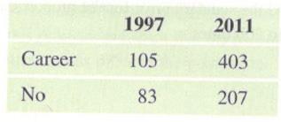
Young Women's Career Goals Are the career goals of young women changing? A Pew Poll asked young women about the importance they place on having a high-paying career or profession. Those women who said being successful in a high-paying career is "one of the most important things" or "very important" in their lives are included in the row labeled Career in the table. Pew asked this question in 1997 and again in 2011.
a. Find and compare the sample proportions of those who had high-paying career goals in 2011 and those who had such goals in 1997.
b. Find a
Want to see the full answer?
Check out a sample textbook solution
Chapter 7 Solutions
Introductory Statistics (2nd Edition)
Additional Math Textbook Solutions
Pathways To Math Literacy (looseleaf)
Precalculus: Mathematics for Calculus (Standalone Book)
College Algebra Essentials (5th Edition)
Elementary Statistics ( 3rd International Edition ) Isbn:9781260092561
APPLIED STAT.IN BUS.+ECONOMICS
University Calculus: Early Transcendentals (4th Edition)


- Selon une économiste d’une société financière, les dépenses moyennes pour « meubles et appareils de maison » ont été moins importantes pour les ménages de la région de Montréal, que celles de la région de Québec. Un échantillon aléatoire de 14 ménages pour la région de Montréal et de 16 ménages pour la région Québec est tiré et donne les données suivantes, en ce qui a trait aux dépenses pour ce secteur d’activité économique. On suppose que les données de chaque population sont distribuées selon une loi normale. Nous sommes intéressé à connaitre si les variances des populations sont égales.a) Faites le test d’hypothèse sur deux variances approprié au seuil de signification de 1 %. Inclure les informations suivantes : i. Hypothèse / Identification des populationsii. Valeur(s) critique(s) de Fiii. Règle de décisioniv. Valeur du rapport Fv. Décision et conclusion b) A partir des résultats obtenus en a), est-ce que l’hypothèse d’égalité des variances pour cette…arrow_forwardAccording to an economist from a financial company, the average expenditures on "furniture and household appliances" have been lower for households in the Montreal area than those in the Quebec region. A random sample of 14 households from the Montreal region and 16 households from the Quebec region was taken, providing the following data regarding expenditures in this economic sector. It is assumed that the data from each population are distributed normally. We are interested in knowing if the variances of the populations are equal. a) Perform the appropriate hypothesis test on two variances at a significance level of 1%. Include the following information: i. Hypothesis / Identification of populations ii. Critical F-value(s) iii. Decision rule iv. F-ratio value v. Decision and conclusion b) Based on the results obtained in a), is the hypothesis of equal variances for this socio-economic characteristic measured in these two populations upheld? c) Based on the results obtained in a),…arrow_forwardA major company in the Montreal area, offering a range of engineering services from project preparation to construction execution, and industrial project management, wants to ensure that the individuals who are responsible for project cost estimation and bid preparation demonstrate a certain uniformity in their estimates. The head of civil engineering and municipal services decided to structure an experimental plan to detect if there could be significant differences in project evaluation. Seven projects were selected, each of which had to be evaluated by each of the two estimators, with the order of the projects submitted being random. The obtained estimates are presented in the table below. a) Complete the table above by calculating: i. The differences (A-B) ii. The sum of the differences iii. The mean of the differences iv. The standard deviation of the differences b) What is the value of the t-statistic? c) What is the critical t-value for this test at a significance level of 1%?…arrow_forward
- Compute the relative risk of falling for the two groups (did not stop walking vs. did stop). State/interpret your result verbally.arrow_forwardMicrosoft Excel include formulasarrow_forwardQuestion 1 The data shown in Table 1 are and R values for 24 samples of size n = 5 taken from a process producing bearings. The measurements are made on the inside diameter of the bearing, with only the last three decimals recorded (i.e., 34.5 should be 0.50345). Table 1: Bearing Diameter Data Sample Number I R Sample Number I R 1 34.5 3 13 35.4 8 2 34.2 4 14 34.0 6 3 31.6 4 15 37.1 5 4 31.5 4 16 34.9 7 5 35.0 5 17 33.5 4 6 34.1 6 18 31.7 3 7 32.6 4 19 34.0 8 8 33.8 3 20 35.1 9 34.8 7 21 33.7 2 10 33.6 8 22 32.8 1 11 31.9 3 23 33.5 3 12 38.6 9 24 34.2 2 (a) Set up and R charts on this process. Does the process seem to be in statistical control? If necessary, revise the trial control limits. [15 pts] (b) If specifications on this diameter are 0.5030±0.0010, find the percentage of nonconforming bearings pro- duced by this process. Assume that diameter is normally distributed. [10 pts] 1arrow_forward
- 4. (5 pts) Conduct a chi-square contingency test (test of independence) to assess whether there is an association between the behavior of the elderly person (did not stop to talk, did stop to talk) and their likelihood of falling. Below, please state your null and alternative hypotheses, calculate your expected values and write them in the table, compute the test statistic, test the null by comparing your test statistic to the critical value in Table A (p. 713-714) of your textbook and/or estimating the P-value, and provide your conclusions in written form. Make sure to show your work. Did not stop walking to talk Stopped walking to talk Suffered a fall 12 11 Totals 23 Did not suffer a fall | 2 Totals 35 37 14 46 60 Tarrow_forwardQuestion 2 Parts manufactured by an injection molding process are subjected to a compressive strength test. Twenty samples of five parts each are collected, and the compressive strengths (in psi) are shown in Table 2. Table 2: Strength Data for Question 2 Sample Number x1 x2 23 x4 x5 R 1 83.0 2 88.6 78.3 78.8 3 85.7 75.8 84.3 81.2 78.7 75.7 77.0 71.0 84.2 81.0 79.1 7.3 80.2 17.6 75.2 80.4 10.4 4 80.8 74.4 82.5 74.1 75.7 77.5 8.4 5 83.4 78.4 82.6 78.2 78.9 80.3 5.2 File Preview 6 75.3 79.9 87.3 89.7 81.8 82.8 14.5 7 74.5 78.0 80.8 73.4 79.7 77.3 7.4 8 79.2 84.4 81.5 86.0 74.5 81.1 11.4 9 80.5 86.2 76.2 64.1 80.2 81.4 9.9 10 75.7 75.2 71.1 82.1 74.3 75.7 10.9 11 80.0 81.5 78.4 73.8 78.1 78.4 7.7 12 80.6 81.8 79.3 73.8 81.7 79.4 8.0 13 82.7 81.3 79.1 82.0 79.5 80.9 3.6 14 79.2 74.9 78.6 77.7 75.3 77.1 4.3 15 85.5 82.1 82.8 73.4 71.7 79.1 13.8 16 78.8 79.6 80.2 79.1 80.8 79.7 2.0 17 82.1 78.2 18 84.5 76.9 75.5 83.5 81.2 19 79.0 77.8 20 84.5 73.1 78.2 82.1 79.2 81.1 7.6 81.2 84.4 81.6 80.8…arrow_forwardName: Lab Time: Quiz 7 & 8 (Take Home) - due Wednesday, Feb. 26 Contingency Analysis (Ch. 9) In lab 5, part 3, you will create a mosaic plot and conducted a chi-square contingency test to evaluate whether elderly patients who did not stop walking to talk (vs. those who did stop) were more likely to suffer a fall in the next six months. I have tabulated the data below. Answer the questions below. Please show your calculations on this or a separate sheet. Did not stop walking to talk Stopped walking to talk Totals Suffered a fall Did not suffer a fall Totals 12 11 23 2 35 37 14 14 46 60 Quiz 7: 1. (2 pts) Compute the odds of falling for each group. Compute the odds ratio for those who did not stop walking vs. those who did stop walking. Interpret your result verbally.arrow_forward
- Solve please and thank you!arrow_forward7. In a 2011 article, M. Radelet and G. Pierce reported a logistic prediction equation for the death penalty verdicts in North Carolina. Let Y denote whether a subject convicted of murder received the death penalty (1=yes), for the defendant's race h (h1, black; h = 2, white), victim's race i (i = 1, black; i = 2, white), and number of additional factors j (j = 0, 1, 2). For the model logit[P(Y = 1)] = a + ß₁₂ + By + B²², they reported = -5.26, D â BD = 0, BD = 0.17, BY = 0, BY = 0.91, B = 0, B = 2.02, B = 3.98. (a) Estimate the probability of receiving the death penalty for the group most likely to receive it. [4 pts] (b) If, instead, parameters used constraints 3D = BY = 35 = 0, report the esti- mates. [3 pts] h (c) If, instead, parameters used constraints Σ₁ = Σ₁ BY = Σ; B = 0, report the estimates. [3 pts] Hint the probabilities, odds and odds ratios do not change with constraints.arrow_forwardSolve please and thank you!arrow_forward
 Glencoe Algebra 1, Student Edition, 9780079039897...AlgebraISBN:9780079039897Author:CarterPublisher:McGraw Hill
 Holt Mcdougal Larson Pre-algebra: Student Edition...AlgebraISBN:9780547587776Author:HOLT MCDOUGALPublisher:HOLT MCDOUGAL
 Big Ideas Math A Bridge To Success Algebra 1: Stu...AlgebraISBN:9781680331141Author:HOUGHTON MIFFLIN HARCOURTPublisher:Houghton Mifflin Harcourt